3. The Poisson Counting Process#
A Poisson counting process \(N(t)\) is a continuous time stochastic process that assumes values on the nonnegative integers, and which can be defined in the following ways. Let \(p_n(t) = \text{Prob}\, \{N(t) = n\},\ t \geq 0,\ n = 0,\ 1,\ 2,\ \ldots\). We define \(N(t)\) by a collection of differential equations for \(p_n(t)\):
where \(\lambda > 0\), and \(p_j(0) = 0\) for \(j \geq 1\). These equations can be arranged conveniently in the form of the infinite matrix equation.
The positive parameter \(\lambda\) is called the rate of the process. The solution of this recursive system of differential equations is readily found to be
Evidently, we could define the Poisson counting process by simply starting with the definitions of probabilities
The mean of the Poisson counting process is readily calculated as
or
This formula motivates the interpretation of \(\lambda\) as the rate or arrival rate of the process. Similar calculations show that
which implies that
An example of a realization of a Poisson counting process is given in Fig. 1. The random points in time \(t_1,\ t_2,\ \ldots\) at which \(N(t)\) jumps are called arrival times.
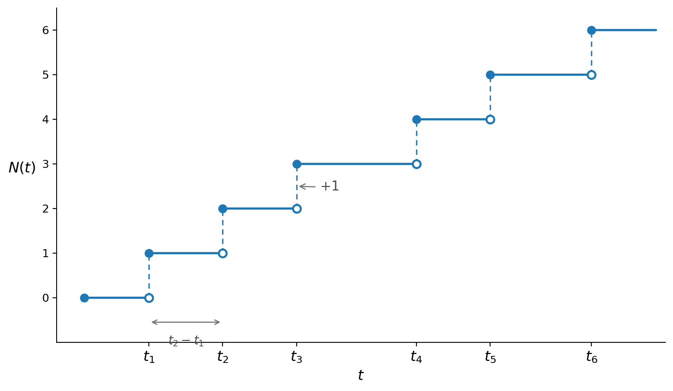
Fig. 1 Figure 1. A realization (sample path) of a Poisson counting process \(N(t)\) with rate \(\lambda\). The process starts at \(N(0) = 0\) and increases by one unit at each random arrival time \(t_1, t_2, \ldots\). It is right-continuous: at an arrival time \(t_i\) it takes the post-jump value \(N(t_i)\) (filled dot), while the pre-jump left limit \(N(t_i^-)\) is shown as an open dot. The interarrival times \(t_i - t_{i-1}\) are independent and exponentially distributed with mean \(1/\lambda\).#
Notice that the event that the first arrival time \(t_1 \leq T_1\) is the event that \(N(T_1) \geq 1\), which is the complement of the event that \(N(T_1) = 0\). Therefore, we have that
which states that the first arrival time is exponentially distributed.
From the above, it follows that a Poisson process \(N(t)\) is characterized by the properties
(i) \(N(0) = 0\)
(ii) For \(t_1 > t_2\),
(iii) If \(t_1 > t_2 > t_3 > t_4\), then \((N(t_1) - N(t_2))\) is statistically independent of \(N(t_3) - N(t_4)\), and \(E(N(t_1) - N(t_2))\, (N(t_3) - N(t_4)) = \lambda^2 (t_1 - t_2)\, (t_3 - t_4)\), so that the expectation of the products of the increments \((N(t_1) - N(t_2))\) and \((N(t_3) - N(t_4))\) is the product of their expectations.
Property (iii) is the “independent increments” property of a Poisson process.
For \(t_1 > t_2\), we have
Assuming again that \(t_1 > t_2 > t_3 > t_4\), and using \(N(t_1) - N(t_3) = (N(t_1) - N(t_2)) + (N(t_2) - N(t_3))\), and \(N(t_2) - N(t_4) = (N(t_2) - N(t_3)) + (N(t_3) - N(t_4))\), we obtain
It follows that
so that the covariance between two increments is proportional to their overlap in time \((t_2 - t_3)\).
Using the preceding formulas, we can calculate the autocorrelation function \(R(t_1,\, t_2)\) and the autocovariance function \(C(t_1,\, t_2)\) for the Poisson process. We find
or
Note that \(\min\, (t_1,\, t_2)\) is the length of overlap of \(N(t_2)\) and \(N(t_1)\). It follows from (14) that
From (15) it follows that \(N(t)\) is mean square continuous. (Why?) From (14), we also have that
or
where \(u(t)\) is the Heaviside unit step function defined by \(u(t) = 1\) for \(t \geq 0,\ u(t) = 0\) for \(t < 0\). It follows from (16) that
where \(\delta(\ \ )\) is the Dirac delta generalized function defined by
for all test functions \(g(t)\) that are continuous at \(t = 0\), and that go to zero sufficiently quickly as \(|t| \to \infty\).
Equation (17) states that \(\partial^2 R(t_1,\, t_2)/\partial t_1 \partial t_2\) does not exist as an ordinary function, so that \(R(t_1,\, t_2)\) is not twice differentiable. It follows that \(N(t)\) is not mean square differentiable, so that \(dN(t)/dt\) does not exist as an ordinary stochastic process.
Although \(dN(t)/dt\) does not exist in the mean square sense, it does exist as a “generalized stochastic process.” The sample paths of the Poisson process can be represented as
where \(\{ t_1,\, t_2,\, \ldots\}\) are the Poisson arrival times and \(u(t)\) is again the Heaviside unit step function. Taking the generalized derivative of the sample path \(N(t)\) and using the definition \(\frac{d}{dt}\, u(t - t_i) = \delta(t - t_i)\), we obtain
so that \(dN(t)/dt\) is a sum of \(\delta\)-impulses at the random arrival times \(t_i\). From our preceding results, it follows that
The zero mean generalized stochastic process \(z(t) - \lambda\), which has autocorrelation function \(\lambda \delta(t_1 - t_2)\) is an example of a white noise. Any stochastic process with an autocorrelation function proportional to \(\delta(t_1 - t_2)\) is known as a white noise. White noise is the elementary building block from which the processes of this book are assembled: it drives the stochastic differential equations of 5. Stochastic Processes Driven by a Poisson Counting Process, reappears in the limit construction of the Wiener process in 6. The Wiener Process, and is the fundamental input \(w(t)\) of the Wold representation in 8. Spectral Densities.
The process \(z(t) = dN(t)/dt\) does not exist as an ordinary stochastic process, but can be regarded as a particular kind of limit point of a process that does exist as an ordinary stochastic process. In particular, for \(\epsilon > 0\), define
where \(N(t)\) is a Poisson counter with rate \(\lambda\). It follows that
where \(k = N(t + \epsilon) - N(t) =\) number of arrivals of the \(N(t)\) process in the interval \((t,\, t + \epsilon)\). Therefore,
Using this Poisson probability distribution, and the above results on moments of a Poisson process, we can deduce that
The function \(\lambda/\epsilon - \lambda |t_1 - t_2|/\epsilon^2\) for \(|t_1 - t_2| \leq \epsilon\) is plotted in Fig. 2, and inscribes a triangle of area \(\lambda\) above the horizontal axis. It is known that the limit as \(\epsilon \to 0\), of the ordinary function \(\max\ (0,\, \frac{\lambda}{\epsilon}\ -\ \frac{\lambda |t_1 - t_2|}{\epsilon^2})\) defines the Dirac delta generalized function with mass \(\lambda\), \(\lambda \delta(t_1 - t_2)\).
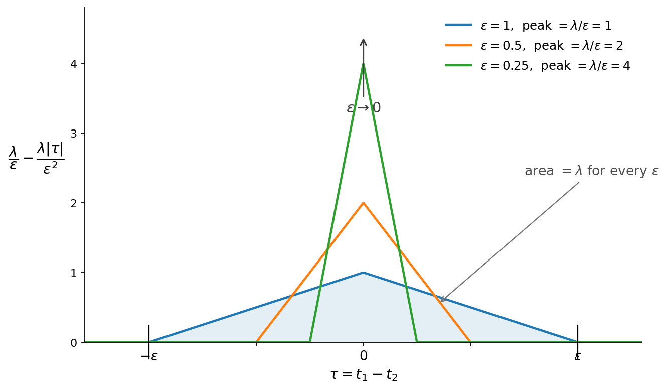
Fig. 2 Figure 2. The triangular function \(\lambda/\epsilon - \lambda|t_1 - t_2|/\epsilon^2\) on \(|t_1 - t_2| \leq \epsilon\), shown for three window widths \(\epsilon\). Each triangle has height \(\lambda/\epsilon\), base \([-\epsilon, \epsilon]\), and area exactly \(\lambda\). As \(\epsilon \to 0\) the triangles become taller and narrower while preserving their area, so in the limit they define the Dirac delta generalized function with mass \(\lambda\), namely \(\lambda\,\delta(t_1 - t_2)\).#
It is a “spike” of “mass” \(\lambda\) at \(t_1 - t_2 = 0\), and is equal to zero for \(t_1 - t_2 \neq 0\).
As an example of one use of the generalized stochastic process \(z(t) = dN(t)/dt\), let \(L(\tau),\ \tau \in [0,\, \infty)\) be a continuous and square integrable function, i.e., \(\int_0^{\infty} L(\tau)^2\, d\tau < +\infty\). Then consider a stochastic process defined by the distributed lag
Substituting \(z(t) = \sum_{i=1}^{\infty}\, \delta(t - t_i)\) and using the definition of the delta generalized function, we find
The process \(Y(t)\) defined by (18) is an ordinary stochastic process, consisting of a sum of the function \(L\) shifted by the random arrival times \(t_i\). Such a process \(Y(t)\) is called shot noise. In 8. Spectral Densities we shall show how to calculate its first and second order moments. Shot noise is the prototype of the lesson made precise in 4. The Concept of “Physical Realizability”: the generalized white noise \(dN/dt\) lives only under the integral sign, while the integrated process \(Y(t)\) is perfectly ordinary.
Exercises#
The following exercises use simulation to illustrate the properties of the Poisson
counting process derived above. They use only numpy and matplotlib.
import numpy as np
import matplotlib.pyplot as plt
The key fact we exploit is that a Poisson process of rate \(\lambda\) can be simulated by drawing independent exponential interarrival times with mean \(1/\lambda\) and accumulating them: the cumulative sums are the arrival times \(t_1, t_2, \ldots\), and \(N(t)\) counts how many arrival times do not exceed \(t\).
def poisson_arrivals(lam, T, rng):
    """Arrival times of a rate-lam Poisson process on the interval [0, T]."""
    times, t = [], 0.0
    while True:
        t += rng.exponential(1.0 / lam)
        if t > T:
            break
        times.append(t)
    return np.array(times)
Exercise 1
Take a Poisson process with rate \(\lambda = 2\).
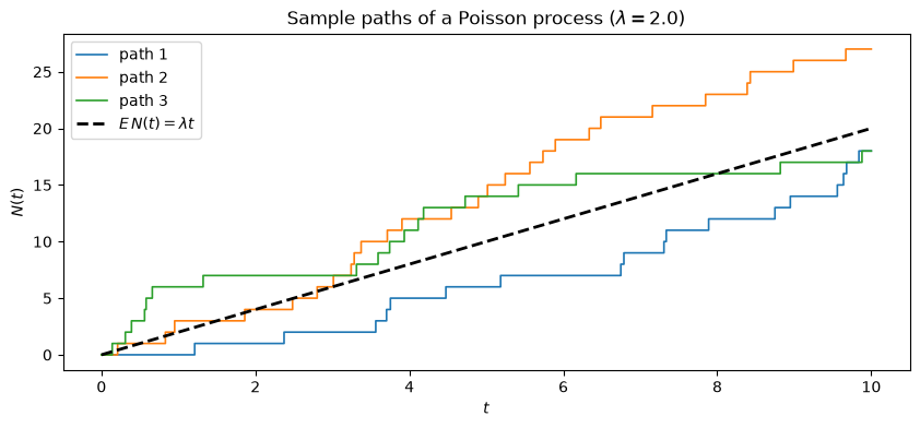
(a) Simulate and plot three sample paths of \(N(t)\) on \([0, 10]\), together with the mean function \(E\,N(t) = \lambda t\).
(b) By simulating many independent paths, verify the moment formulas \(E\,N(T) = \lambda T\) and \(\operatorname{Var} N(T) = \lambda T\) derived in the text. (Recall that \(\operatorname{Var} N(T) = E\,N(T)\) is a signature property of the Poisson distribution.)
Solution to Exercise 1
rng = np.random.default_rng(42)
lam, T = 2.0, 10.0

# (a) three sample paths
grid = np.linspace(0, T, 1000)
fig, ax = plt.subplots(figsize=(10, 4))
for i in range(3):
    arr = poisson_arrivals(lam, T, rng)
    Nt = np.searchsorted(arr, grid, side='right')   # N(t) = #{arrivals <= t}
    ax.step(grid, Nt, where='post', lw=1.2, label=f'path {i+1}')
ax.plot(grid, lam * grid, 'k--', lw=2, label=r'$E\,N(t)=\lambda t$')
ax.set_xlabel('$t$'); ax.set_ylabel('$N(t)$')
ax.set_title(rf'Sample paths of a Poisson process ($\lambda={lam}$)')
ax.legend()
plt.show()
# (b) Monte Carlo check of the first two moments of N(T)
reps = 20_000
counts = np.array([len(poisson_arrivals(lam, T, rng)) for _ in range(reps)])

print(f"E[N(T)]:    simulated {counts.mean():.3f},   theory {lam * T:.3f}")
print(f"Var[N(T)]:  simulated {counts.var():.3f},   theory {lam * T:.3f}")
E[N(T)]:    simulated 20.044,   theory 20.000
Var[N(T)]:  simulated 20.164,   theory 20.000
The simulated mean and variance both sit close to \(\lambda T = 20\), as the theory predicts.
Exercise 2
The text shows that the first arrival time is exponentially distributed, \(\operatorname{Prob}\{t_1 \le T_1\} = 1 - e^{-\lambda T_1}\). More generally, the interarrival times \(t_{i} - t_{i-1}\) of a Poisson process are independent and exponentially distributed with mean \(1/\lambda\).
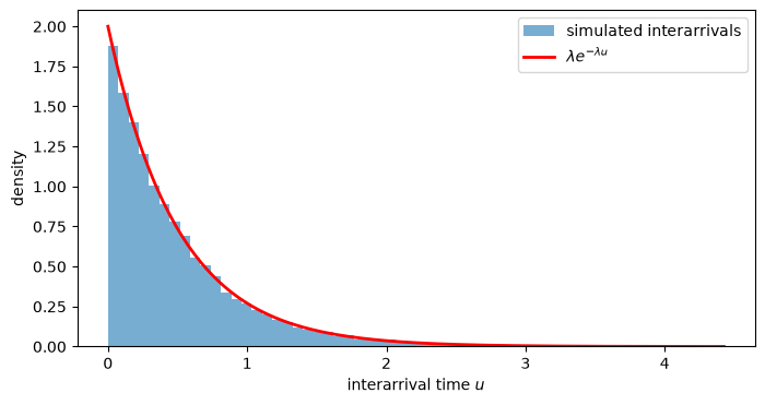
Simulate one long sample path (rate \(\lambda = 2\) on \([0, 5000]\)), extract its interarrival times, and compare their histogram with the exponential density \(\lambda e^{-\lambda u}\). Report the sample mean interarrival time and compare it to \(1/\lambda\).
Solution to Exercise 2
arr = poisson_arrivals(lam, 5000.0, rng)
gaps = np.diff(np.concatenate([[0.0], arr]))   # interarrival times

fig, ax = plt.subplots(figsize=(8, 4))
ax.hist(gaps, bins=60, density=True, alpha=0.6, label='simulated interarrivals')
u = np.linspace(0, gaps.max(), 200)
ax.plot(u, lam * np.exp(-lam * u), 'r-', lw=2, label=r'$\lambda e^{-\lambda u}$')
ax.set_xlabel('interarrival time $u$'); ax.set_ylabel('density')
ax.legend()
plt.show()

print(f"mean interarrival time: simulated {gaps.mean():.4f},  theory {1/lam:.4f}")
mean interarrival time: simulated 0.4993, theory 0.5000
The histogram tracks the exponential density and the mean gap is close to \(1/\lambda = 0.5\), confirming the exponential interarrival property.