23. Temporal Aggregation of Economic Time Series#
Note
This chapter reports and paraphrases Albert Marcet’s chapter “Temporal Aggregation of Economic Time Series” in Rational Expectations Econometrics, edited by Lars Peter Hansen and Thomas J. Sargent (Boulder: Westview Press, 1991). We retell Marcet’s analysis in our own words, compress his proofs and his catalogue of simulations, and add numerical illustrations. We also read his results as an application of the earlier chapters: the \(L^2\) projection theory of Chapter 19, the sum-of-exponentials kernels of Chapter 11, the continuous-time prediction formulas of Chapter 12, and the local unpredictability of Chapter 13. The substantive claims and constructions are Marcet’s. The framing in terms of the earlier chapters is ours, and phrasings such as “Marcet shows” keep the attribution clear.
Introduction#
19. Prediction Formulas for Continuous Time Linear Rational Expectations Models developed the theory of linear prediction for a process observed continuously in time. Working in the Hilbert space \(L^2\), it represented a stationary process as a convolution of a square-integrable kernel with an orthogonal random measure, exploited the isometry between functions in \(L^2\) and the random variables they generate, and showed that the least-squares forecast is obtained, on the function side, by a simple operation on the kernel.
Economic variables, however, are almost never observed continuously. We have quarterly observations on GNP, monthly observations on many prices, and so on, even though there is no reason to think the economy moves only at the dates on which we happen to collect data. Temporal aggregation is the name for this situation: an underlying process evolves in continuous time, but we observe it only at discrete intervals. Marcet’s chapter studies what is lost in that step.
Marcet keeps the continuous-time framework of Chapter 19: a random measure with orthogonal, second-moment-stationary increments, and processes built as convolutions of \(L^2\) kernels with that measure. He asks how the fundamental moving-average representation (MAR, or Wold representation) of the sampled process relates to the MAR of the underlying continuous process. Because the MAR summarizes the entire linear forecasting structure of a process, it is the natural object through which to view the effects of sampling.
The questions Marcet focuses on are these. Which features of the continuous MAR are captured by the discrete MAR, and which are systematically distorted? How are the one-step-ahead prediction errors in continuous and discrete time related? What happens when, in addition to sampling, the data are averaged over the sampling interval? And can the continuous model be recovered by sampling ever more finely? The answers are useful in practice: if an estimated discrete-time model has features hard to reconcile with economic theory, one would like to know whether temporal aggregation alone could have produced them, and if so, whether the remedy is finer data or a continuous-time structural model estimated from discrete data through the cross-equation restrictions of a rational expectations model (Hansen and Sargent 1991).
The whole analysis turns on a single idea, and it is exactly the projection idea of Chapter 19: the discrete-time forecast, viewed on the function side, is the projection of the continuous-time kernel onto the closed subspace generated by its integer shifts. Almost everything Marcet proves is a consequence of that one observation. The discontinuities that a one-sided continuous-time kernel carries open up possibilities for the sampled kernel. The smooth, two-sided distributed lag problems that Sims (1971) and Geweke (1978) studied have no counterpart to them. The numerical illustrations below display them.
1. Setup: continuous and sampled moving-average representations#
Marcet takes an \(n\)-dimensional continuous-time process \(y\), mean zero, covariance stationary, linearly indeterministic, with finite variances. As in Chapter 19, random variables are treated as elements of a Hilbert space with inner product \(E(xz)\), and \(H_y(t)\) denotes the closed linear span of \(\{y_i(s): s \le t\}\), the information available through time \(t\). The projection \(\eta(y(t+\alpha)\mid H_y(t))\) is the best linear predictor of \(y(t+\alpha)\) given that information. These assumptions deliver the fundamental moving-average representation
where \(a : \mathbb{R} \to \mathbb{R}^{n\times m}\) is square integrable and \(\zeta\) is an \(m\)-dimensional orthonormal random measure. The isometry of Chapter 19 states that for square-integrable \(f, g\),
from which \(E[y(t) y(t-s)'] = \int_0^\infty a(u)\,a(u-s)'\, du\), and the forecast reads off the kernel directly, \(\eta(y(t)\mid H_y(t-\alpha)) = \int_\alpha^\infty a(u)\,\zeta(t-du)\). This last formula is the continuous-time counterpart of the annihilation-operator prediction formulas of Chapter 12: forecasting \(\alpha\) periods back simply truncates the kernel below \(\alpha\).
From \(y\) Marcet forms the sampled process \(Y(t) = y(t)\) for integer \(t\). Because \(H_Y(s) \subset H_y(s)\), the sampled process inherits stationarity and linear regularity, so it too has a (discrete) MAR
with \(\epsilon\) an \(n\)-dimensional white noise. (Extending \(a\) and \(A\) by zero to negative arguments, (234) and (235) are convolutions \(y = a*\zeta\) and \(Y = A*\epsilon\).) Unlike the continuous innovations \(\zeta\), the components of \(\epsilon\) need not be contemporaneously uncorrelated. Assuming \(y\) has a spectral density that is positive definite almost everywhere, \(Y\) is full rank as well, since its spectral density is given by the folding formula of Chapter 17,
The aliasing that the folding formula encodes at the level of spectra will reappear below at the level of kernels.
2. The sampled innovation as a projection#
Normalize the discrete MAR so that \(\epsilon(t) = Y(t) - \eta(Y(t)\mid H_Y(t-1))\) is the one-step-ahead innovation of the sampled process. Marcet’s starting point is a decomposition of this innovation into a continuous-time piece and a “reconstruction error,”
The first term is the continuous-time one-step innovation, the part of \(y(t)\) that the continuous past does not forecast; it is orthogonal to \(H_y(t-1)\). The second term, \(B_t\), lives inside \(H_y(t-1)\), so the two are orthogonal. In words, the discrete innovation is the continuous innovation plus the error one makes in reconstructing the continuous-time forecast from sampled data. By the law of iterated projections, \(\eta(Y(t)\mid H_Y(t-1)) = \eta[\,\eta(y(t)\mid H_y(t-1))\mid H_Y(t-1)\,]\), so \(B_t\) is exactly the error in predicting the continuous forecast from the samples; the sampled innovation is large, relative to the continuous one, precisely when the continuous-time forecast is hard to recover from samples.
Read the first term through Chapter 13. There it was shown that a process fails to be mean square differentiable exactly when its Wold kernel does not vanish at the origin, \(a(0)\neq 0\). It is then locally unpredictable. The continuous one-step innovation \(\int_0^1 a(u)\,\zeta(t-du)\) inherits its size from the behaviour of \(a\) near \(u=0\); a kernel with \(a(0)\neq 0\) delivers a genuinely unpredictable continuous innovation, while a smooth kernel with \(a(0)=0\) makes the process locally predictable. We shall see this distinction govern how badly sampling distorts the dynamics.
Since \(B_t \in H_\zeta(t-1)\), Marcet writes the whole innovation as a convolution \(\epsilon(t) = \int_0^\infty c(u)\,\zeta(t-du)\) for a kernel \(c\) that equals \(a\) on \([0,1)\). Writing the discrete forecast itself as \(\eta(Y(t)\mid H_Y(t-1)) = \int_1^\infty h(u)\,\zeta(t-du)\), the weighting kernel is \(c = a - h\). The function \(h\) has a clean description in \(L^2\), and identifying it is the crux of the whole theory. Let \(L^2_n\) be the row-vector functions \(f:\mathbb{R}\to\mathbb{R}^n\) with inner product \(\langle f,g\rangle = \int f(u) g(u)'\, du\), let \(a_i\) be the \(i\)-th row of \(a\), and let
be the closed span of the integer-lagged rows of \(a\). Marcet’s central result identifies \(h\) with a projection.
Proposition 1 (Marcet)
For each \(i\), \(\;h_i = \eta(a_i\mid A)\): the discrete-forecast kernel is the projection of the continuous kernel \(a_i\) onto the closed span of its own integer shifts.
The proof is a direct transcription of the Chapter 19 isometry. Using \(\int_0^\infty a_j(u-k)\,\zeta(t-du) = Y_j(t-k)\), the orthogonality on the function side, \(\int_0^\infty [a_i(u)-h_i(u)]\,a_j(u-k)'\, du = 0\) for all \(k\ge 1\), is the same statement as the orthogonality of the discrete one-step innovation to past \(Y\)’s, \(\operatorname{cov}[\,Y_i(t)-\eta(Y_i(t)\mid H_Y(t-1)),\,Y_j(t-k)\,] = 0\). Closedness of \(A\) then puts \(h_i\) inside \(A\), and the projection theorem does the rest. This is the projection idea of Chapter 19 carried out on the kernel: the discrete forecast corresponds to approximating \(a_i\) as closely as possible by a combination \(\sum_k \lambda_k\, a(\cdot-k)\) of its own unit shifts, and the residual of that approximation is \(c_i = a_i - \eta(a_i\mid A)\).
A pair of equivalences, used repeatedly below, falls straight out of Proposition 1.
Proposition 2 (Marcet)
For each \(i\), the following are equivalent: (i) \(c_i(u)=0\) for almost every \(u\ge 1\); (ii) the discrete and continuous one-step forecasts of \(y_i\) coincide, \(\eta(Y_i(t)\mid H_Y(t-1)) = \eta(y_i(t)\mid H_y(t-1))\); (iii) \(a_i(u) = \eta(a_i\mid A)(u)\) for almost every \(u\ge 1\), so that on \([1,\infty)\) the kernel reproduces itself under its own shifts.
3. Marcet’s formula for the discrete kernel, and the role of discontinuities#
With \(c\) in hand, Marcet expresses the discrete MAR coefficients in terms of the continuous kernel.
Proposition 3 (Marcet)
The matrices in the discrete MAR (235) are
The proof is one line of the isometry: with \(V = E[\epsilon\epsilon'] = \int_0^\infty c c'\), \(A_k V = E[Y(t+k)\epsilon(t)'] = \int_0^\infty a(u+k)\,c(u)'\, du\).
Proposition 3 says that each discrete coefficient \(A_k\) is a weighted average of the continuous kernel \(a\) over \([k,\infty)\), with the residual \(c\) supplying the weights. Two facts shape those weights. First, \(c = a\) on \([0,1)\) while every function in \(A\) vanishes there, so the projection contributes nothing on the first interval. Second, on \([1,\infty)\) the size of \(c\) is governed by
the gap between how well one can predict \(y_i\) from discrete and from continuous data. This single number governs everything: when the gap is small, \(c\) is concentrated on \([0,1)\), so \(A_k\) leans on \(a\) over \([k,k+1)\) and the discrete kernel resembles the continuous one (Fig. 7); when the gap is large, the discrete MAR can be badly distorted.
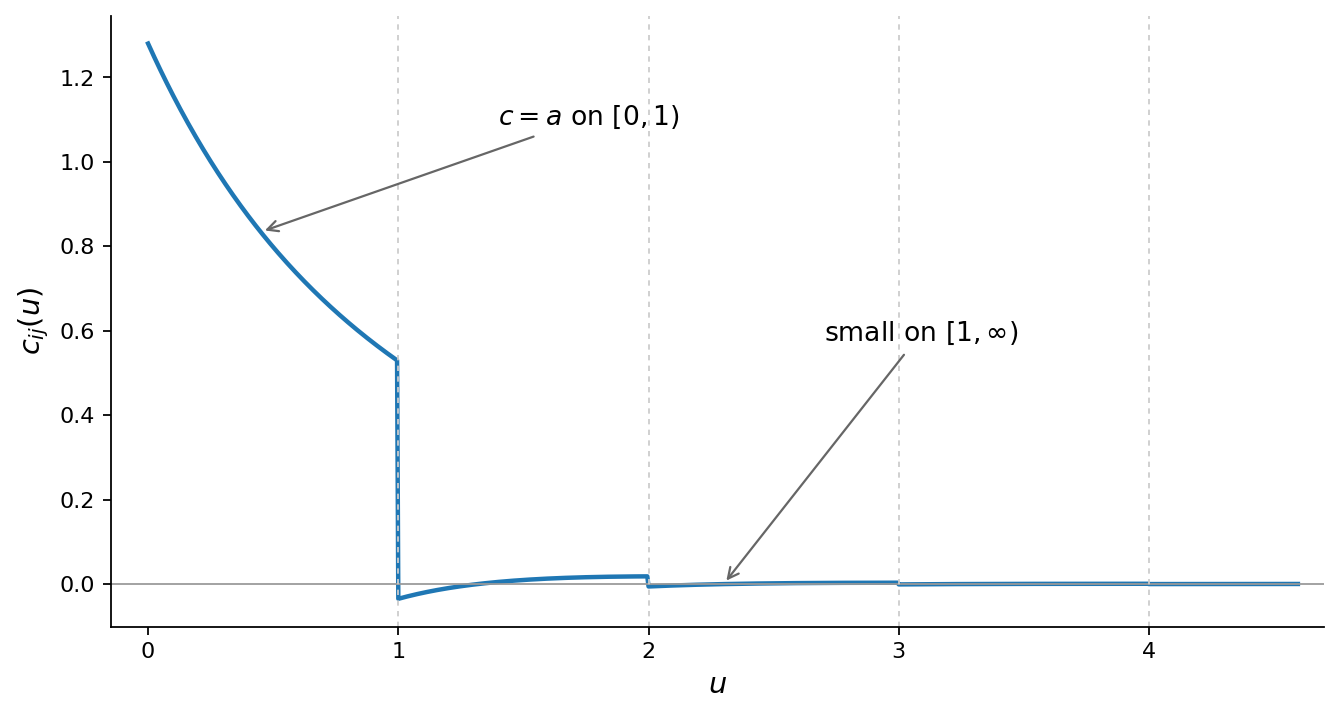
Fig. 7 The weighting kernel \(c\). It coincides with \(a\) on \([0,1)\) and is small on \([1,\infty)\) when discrete data predict almost as well as continuous data.#
A systematic inflation. Even when the discrete kernel resembles the continuous one, Marcet shows that sampling inflates the leading coefficients. Because \(Y\) is forecastable no better than \(y\), for every \(\nu\), \(\operatorname{var}(Y_i(t)-\eta(Y_i(t)\mid H_Y(t-\nu))) \ge \operatorname{var}(y_i(t)-\eta(y_i(t)\mid H_y(t-\nu)))\), which in the univariate case reads \(\sigma_\epsilon^2\sum_{k=0}^{\nu-1}A_k^2 \ge \int_0^\nu a^2\). The discrete MAR must pack into a few coefficients the variance that the continuous MAR spreads over an interval, so its early coefficients are too large in absolute value. This is the mirror image of Chapter 13’s lesson about packing: a continuous innovation with \(a(0)\neq 0\) carries real one-step surprise, and the discrete representation has to absorb it up front.
Contamination. Formula (238) also shows that the \(i\)-th row of \(A_k\) depends, through \(a\) and \(c\), on all rows of the continuous kernel; each sampled variable’s MAR mixes the continuous dynamics of every variable in the system. Geweke (1978) called this contamination. It is present even when discrete and continuous forecasts coincide, and vanishes only when \(a_{ij}\equiv 0\) for \(i\neq j\).
Why discontinuities matter. Here is Marcet’s decisive contrast with the distributed-lag problems of Sims and Geweke. There the aggregating kernel is two-sided and continuous, and its effect is to shrink the leading discrete coefficients. Marcet’s weighting kernel \(c\) is instead one-sided and, in general, discontinuous. To see the discontinuity, suppose \(a\) is univariate and continuous except at the origin, with \(a(0)\neq 0\), the locally-unpredictable case of Chapter 13. Since \(c(u) = a(u) - \sum_{k\ge 1}\lambda_k\, a(u-k)\), at an integer \(\nu\) the term \(k=\nu\) contributes \(\lambda_\nu\, a(0)\), a jump, because \(a\) jumps at \(0\); the remaining terms are continuous there, so \(c\) inherits a jump at every integer. These jumps, and the one-sidedness, are exactly what give the sampled MAR possibilities the smooth distributed-lag kernel never had. They include the inflation just described and, as the examples now show, the ability for very different continuous kernels to produce identical discrete ones.
Marcet’s examples#
A handful of one-variable examples, all Marcet’s, show how Proposition 1, Proposition 2, and Proposition 3 are used, and when distortions are large or small. The kernels \(e^{-\lambda u}\) and sums of exponentials are the rational-spectral-density kernels of Chapter 11.
Example 4 (Continuous AR(1), no distortion)
Let \(a(u) = e^{-\lambda u}\), \(\lambda>0\). Since \(e^{-\lambda}a(u-1) = a(u)\) for all \(u\ge 1\), the projection reproduces \(a\) exactly on \([1,\infty)\), so \(c=0\) there (Proposition 2). Marcet’s formula collapses to \(A_k = e^{-\lambda k} = a(k)\): the sampled process is a discrete AR(1) and its MAR is just the continuous kernel sampled at the integers. A scale-invariant exponential is the one kernel that sampling leaves alone.
Example 5 (A smooth kernel that is nonetheless distorted)
Take \(a(u) = e^{-\lambda_1 u}+e^{-\lambda_2 u}\) with \(\lambda_1\neq\lambda_2\). Marcet notes that \(\int_1^\infty\|c\|^2 > 0\): were it zero, Proposition 2 would supply a constant \(\mu\) with \(\mu\,a(u-1)=a(u)\) for all \(u\ge 1\). Evaluating at \(u=1\) gives \(\mu = a(1)/a(0) = (e^{-\lambda_1}+e^{-\lambda_2})/2\), and then \(u=2\) forces \((e^{-\lambda_1}+e^{-\lambda_2})^2 = 2(e^{-2\lambda_1}+e^{-2\lambda_2})\), i.e. \((e^{-\lambda_1}-e^{-\lambda_2})^2 = 0\), impossible when \(\lambda_1 \neq \lambda_2\). So an innocuous sum of two exponentials already produces a distorted discrete MAR. More sharply (Hansen and Sargent 1991): if \(a\) is continuous with \(a(0)\neq 0\) and the sampled process has an autoregressive representation with \(c=0\) on \([1,\infty)\), that representation must be first order. Anything richer than a continuous AR(1) is distorted by sampling.
Example 6 (Good prediction, bad shape)
Let \(|a(u)| = e^{-\lambda u}\) but let \(a\) change sign within each unit interval, so \(a\) oscillates while its envelope decays. Again \(e^{-\lambda}a(u-1) = a(u)\) for \(u\ge 1\), so by Proposition 2 the discrete and continuous forecasts coincide and \(A_k = e^{-\lambda k} > 0\). That is the same discrete MAR as the smooth AR(1) of Example 4. The within-interval oscillations are completely invisible to the sampled MAR. Even when discrete data predict as well as continuous data, the discrete MAR can look nothing like the continuous one. This is the kernel-level face of the aliasing of Chapter 17.
Example 7 (\(a(0)=0\) need not mean distortion)
Example 5 might suggest a kernel with \(a(0)=0\) always approximates poorly, but Marcet shows otherwise. Take any \(a\) continuous on \([0,1]\) with \(a(0)=a(1)=0\) and extend it by \(a(u)=\ell\,a(u-1)\), \(0<\ell<1\), for \(u\ge 1\). Then \(\ell\,a(u-1)=a(u)\) on \([1,\infty)\), Proposition 2 applies, and \(Y\) is a discrete AR(1). What matters for distortion is not the value \(a(0)\) but whether \(a\) on \([1,2)\) is a scaled copy of \(a\) on \([0,1)\).
Example 4, Example 6, and Example 7 already exhibit the aliasing problem: different continuous kernels all generating the same sampled process (a discrete AR(1)). The continuous kernel cannot be recovered from discrete data without further restrictions. 17. Discrete Sampling: The Folding Formula and 22. The Dimensionality of the Aliasing Problem in Models with Rational Spectral Densities make the same point.
A numerical illustration of Marcet’s point#
To see Marcet’s discontinuity theme concretely, we compute, for a scalar kernel \(a\), the weighting kernel \(c = a - \eta(a\mid A)\) and the discrete coefficients \(A_k\) of (238). The projection \(\eta(a\mid A)\) is, by Proposition 1, the least-squares approximation of \(a\) by a combination \(\sum_{k\ge 1}\lambda_k\, a(\cdot-k)\) of its own unit shifts; on a fine grid this is an ordinary linear least-squares problem.
import numpy as np
import matplotlib.pyplot as plt

def discrete_MAR(a_func, U=40.0, du=0.002, K=35, n_coef=7):
    """Given a one-sided continuous kernel a_func, return the weighting kernel c
    and the discrete MAR coefficients A_k of Marcet's {prf:ref}`prop-marcet-3`."""
    u = np.arange(0.0, U, du)
    a = a_func(u)
    # columns a(u-k), k=1..K  (a is one-sided: zero for negative argument)
    shifts = [np.where(u - k >= 0, a_func(np.clip(u - k, 0, None)), 0.0) for k in range(1, K + 1)]
    M = np.column_stack(shifts)
    lam, *_ = np.linalg.lstsq(M, a, rcond=None)   # projection onto span of integer shifts
    c = a - M @ lam                               # weighting kernel  c = a - eta(a | A)
    V = np.sum(c * c) * du                         # innovation variance  ∫ c^2
    A = np.array([np.sum(a_func(u + k) * c) * du / V for k in range(n_coef)])
    return u, a, c, A

lam = 0.5
u,  a_ar,  c_ar,  A_ar  = discrete_MAR(lambda u: np.exp(-lam * u))                                   # AR(1)
_,  a_osc, c_osc, A_osc = discrete_MAR(lambda u: np.exp(-lam * u) * np.sign(np.sin(2*np.pi*u)+1e-12)) # oscillating
ut, a_2e,  c_2e,  A_2e  = discrete_MAR(lambda u: np.exp(-0.4 * u) + np.exp(-1.2 * u))                 # two-exponential

print("discrete MAR coefficients A_k:")
print("  AR(1)        :", np.round(A_ar, 4))
print("  oscillating  :", np.round(A_osc, 4), " (identical to AR(1):",
      np.allclose(A_ar, A_osc, atol=1e-3), ")")
print("  two-exp      :", np.round(A_2e, 4))
print("  two-exp a(k)/a(0):", np.round((np.exp(-0.4*np.arange(7)) + np.exp(-1.2*np.arange(7)))/2, 4),
      " <- A_k sits above these (inflation)")
discrete MAR coefficients A_k:
  AR(1)        : [1.     0.6065 0.3679 0.2231 0.1353 0.0821 0.0498]
  oscillating  : [1.     0.6065 0.3679 0.2231 0.1353 0.0821 0.0498]  (identical to AR(1): True )
  two-exp      : [1.     0.5136 0.297  0.1849 0.1197 0.0789 0.0525]
  two-exp a(k)/a(0): [1.     0.4858 0.27   0.1643 0.1051 0.0689 0.0457]  <- A_k sits above these (inflation)
fig, (axL, axR) = plt.subplots(1, 2, figsize=(13, 5))

# Left: two very different continuous kernels with the SAME discrete MAR (kernel aliasing)
axL.axhline(0, color='k', lw=0.6)
axL.plot(u, a_ar, 'C0', lw=2, label=r'AR(1) kernel $e^{-\lambda u}$')
axL.plot(u, a_osc, 'C1', lw=1.5, alpha=0.8,
         label=r'oscillating kernel $e^{-\lambda u}\,\mathrm{sgn}\sin 2\pi u$')
axL.stem(np.arange(7), A_ar, linefmt='C3-', markerfmt='C3o', basefmt=' ',
         label=r'discrete MAR $A_k$ (same for both)')
axL.set_xlim(0, 4); axL.set_xlabel('$u$'); axL.set_ylabel('kernel')
axL.set_title('Different continuous kernels, identical sampled MAR')
axL.legend(fontsize=8.5)

# Right: a distorted case -- A_k inflated above the (normalized) sampled continuous kernel
norm = (np.exp(-0.4*ut) + np.exp(-1.2*ut)) / 2.0
axR.axhline(0, color='k', lw=0.6)
axR.plot(ut, norm, 'C0', lw=2, label=r'$a(u)/a(0)$  (two exponentials)')
axR.plot(ut, c_2e, 'C2', lw=1, alpha=0.6, label=r'weighting kernel $c$ (mass spills past $u=1$)')
axR.stem(np.arange(7), A_2e, linefmt='C3-', markerfmt='C3o', basefmt=' ',
         label=r'discrete MAR $A_k$ (inflated)')
axR.set_xlim(0, 4); axR.set_xlabel('$u$')
axR.set_title('Distortion: the discrete MAR inflates the early coefficients')
axR.legend(fontsize=8.5)
plt.tight_layout(); plt.show()
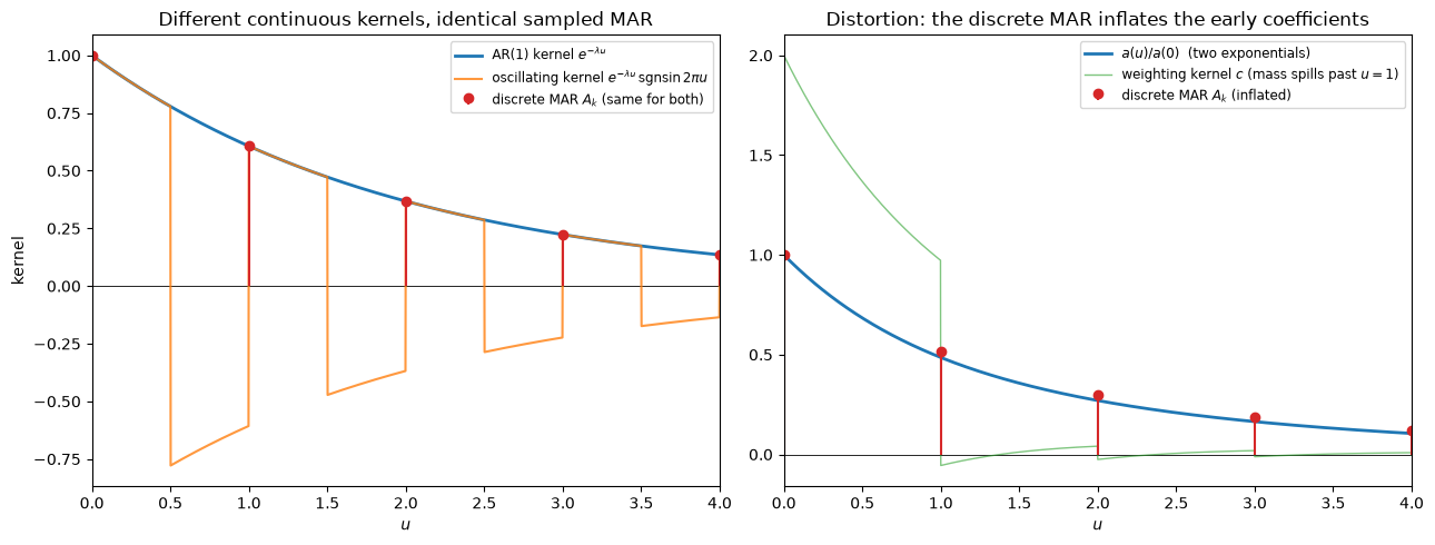
The left panel shows Marcet’s aliasing point: the smooth AR(1) kernel and a kernel that changes sign within every sampling interval are utterly different continuous-time models, yet they yield byte-for-byte the same discrete MAR \(A_k = e^{-\lambda k}\). The discontinuous, within-interval structure does not survive sampling. It is the kernel-level analogue of the spectral folding of (236). The right panel shows the other face of the same phenomenon: for a kernel whose shape on \([1,2)\) is not a scaled copy of its shape on \([0,1)\), the weighting kernel \(c\) carries mass past \(u=1\), and the discrete coefficients \(A_k\) rise above the normalized continuous values \(a(k)/a(0)\), the systematic inflation. Both effects are absent for the smooth, scale-invariant exponential and are made possible exactly by the kind of within-interval variation a one-sided, discontinuous kernel can carry.
4. Granger causality under sampling#
Marcet next shows that sampling generally creates Granger causality. For a bivariate continuous process in which \(y_2\) does not Granger-cause \(y_1\), the sampled \(Y_2\) will typically help predict \(Y_1\), because the discrete forecast of \(Y_1\) implicitly involves the values of \(y_1\) between sampling dates, and past \(Y_2\) can help predict those intermediate values. There is, however, a clean sufficient condition for non-causality to survive. It is the familiar one, that discrete data forecast as well as continuous data.
Proposition 4 (Marcet)
If \(\eta(y_1(t)\mid H_y(t-1)) = \eta(Y_1(t)\mid H_Y(t-1))\) (discrete and continuous one-step forecasts of \(y_1\) coincide) and \(y_2\) fails to Granger-cause \(y_1\), then \(Y_2\) fails to Granger-cause \(Y_1\).
Intuitively, when discrete data predict \(y_1\) as well as continuous data, there is nothing to be gained from reconstructing the intermediate values of \(y_1\), and hence no room for \(Y_2\) to enter.
Marcet also shows the effect can run the other way. One can build continuous systems in which \(y_2\) does Granger-cause \(y_1\) yet the sampled \(Y_2\) does not Granger-cause \(Y_1\): it suffices that the cross-covariances \(\operatorname{cov}(Y_1(t), Y_2(t-s))\) vanish at all integer lags \(s\ge 1\) while the continuous cross-kernels are not identically zero (Fig. 8). What such constructions share is that most of the variance of \(Y_1(t)\) originates in innovations within the last sampling interval. And unit-averaging can reverse direction in yet another way: for \(a_{11}(u)=e^{-\lambda u}\), \(a_{21}(u)=Ke^{-\lambda u}\), \(a_{12}\equiv 0\), continuous-time non-causality of \(y_2\) for \(y_1\) survives point sampling (Proposition 4), but if \(y_1\) is averaged while \(y_2\) is sampled, the smoothing of \(a_{11}\) destroys the alignment and \(Y_2\) comes to Granger-cause \(Y_1\). Whether non-causality survives aggregation thus depends not only on the continuous dynamics but on exactly how the data are collected.
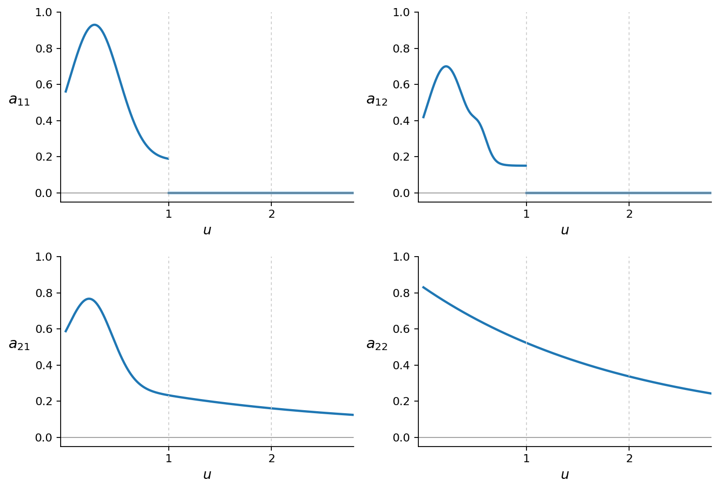
Fig. 8 Continuous-time kernels (Marcet) for which \(y_2\) Granger-causes \(y_1\) but the sampled \(Y_2\) does not Granger-cause \(Y_1\): the cross-covariances of \(Y_1\) with past \(Y_2\) vanish at all integer lags.#
5. Unit-averaged data#
Often data are not point samples but averages over the sampling interval, a monthly figure being the average of underlying weekly values. Marcet treats the case in which the first variable is observed as a unit average and the second as a point sample, \(Y_1(t) = \int_0^1 y_1(t-s)\, ds\), \(Y_2(t) = y_2(t)\). The averaged variable is itself a point sample of the filtered continuous process \(\tilde y_1(t) = \int_0^1 y_1(t-s)\, ds = (\ell * y_1)(t)\), where \(\ell\) is the indicator of \([0,1)\). Passing to the frequency domain exactly as in Chapter 8, the filtered spectral density is \(\hat\ell(\omega)\,\hat a_1(\omega)\,[\hat\ell(\omega)\,\hat a_1(\omega)]'\), and because \(\ell\) contributes no right-half-plane zeros, \(\ell * a_1\) is itself the fundamental MAR kernel of \(\tilde y_1\). The transform \(\hat\ell(s) = (1 - e^{-s})/s\) has its zeros at \(s = 2\pi i k\), \(k \neq 0\), on the imaginary axis itself:
Averaging therefore smooths the kernel and shifts its mass one unit to the right. Marcet records the smoothing precisely.
Proposition 5 (Marcet)
If \(a_{ij}\in L^1\) then \(\tilde a_{ij}\) is continuous; if in addition \(a_{ij}\in C^s\) then \(\tilde a_{ij}\in C^{s+1}\).
The proof is immediate: with \(F(x)=\int_{-\infty}^x a_{ij}\), \(\tilde a_{ij}(u)=F(u)-F(u-1)\). In particular \(\tilde a(0)=0\) always. Through the eyes of Chapter 13, averaging turns a possibly locally-unpredictable process (\(a(0)\neq 0\)) into a mean square continuous, more predictable one (\(\tilde a(0)=0\)). But as Example 5 warned, kernels with \(a(0)=0\) tend to produce distorted discrete MARs. The projection \(h(u)\approx\mu\,a(u-1)\) leaves a large residual on \([1,2)\) relative to \([0,1)\) (Fig. 9). Smoothing the kernel buys predictability at the cost of representation.
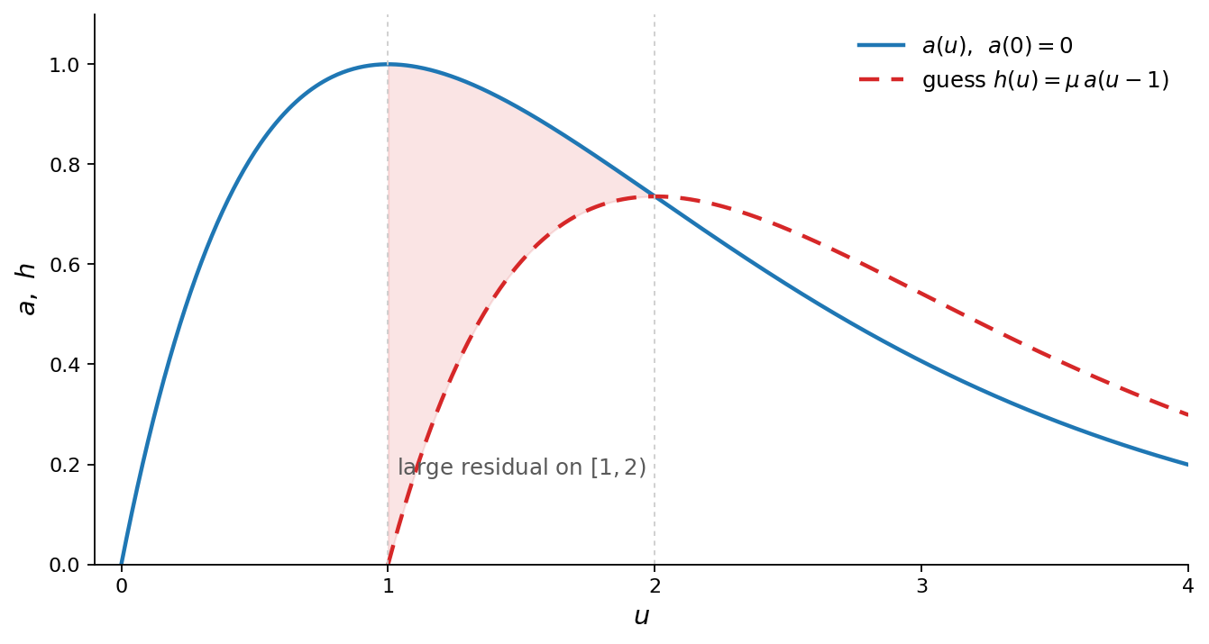
Fig. 9 A continuous kernel \(a\) with \(a(0)=0\) (as produced by averaging) and its one-lag projection \(h\). The residual \(c=a-h\) is large on \([1,2)\) relative to \([0,1)\), signalling a distorted discrete MAR.#
Mixing averaged and sampled data. Marcet’s most useful applied warning concerns systems in which one series is unit-averaged and another point-sampled, a common situation when two series are recorded at different frequencies. He shows that this practice systematically overstates the importance of the sampled variable. The reason is again the projection picture: predicting the averaged \(Y_1\) from its own past means approximating the smooth kernel \(\tilde a_1\) (which starts from \(\tilde a_1(0)=0\)) by a combination of its own integer shifts, and shifted copies that also start from zero cannot build up the mass that \(\tilde a_1\) has just after each integer. The own-variable weights therefore shrink, and the burden of prediction shifts onto the sampled variable \(Y_2\). (For the sampled variable, with \(a_1(0)\neq 0\), the same self-approximation works much better.) Marcet supports the claim with simulations: several discrete bivariate AR(2) processes were aggregated three ways: both sampled, both averaged, and mixed, the first averaged and the second sampled. A VAR variance decomposition was computed for each. In the most dramatic case the share of variance attributed to \(Y_1\) collapsed once it was averaged while \(Y_2\) was sampled (under one Choleski ordering, from 85% to a fraction of a percent). One of the six simulated decompositions moved the other way, as one expects of a heuristic rather than a theorem, but the weight of the evidence is clear: mixing averaged with sampled data biases the analysis toward the sampled variables.
6. Sampling ever more finely#
Finally Marcet asks whether the continuous model is recovered as the sampling interval shrinks. For \(\delta>0\) let \(Y^\delta(t) = y(t\delta)\), indexing information sets by real time so that models with different \(\delta\) can be compared at a fixed real horizon. The forecasts converge under very general conditions.
Proposition 6 (Marcet)
For any \(\alpha>0\), \(t\), and \(i\), \(\eta(Y_i^\delta(t/\delta)\mid H_{Y^\delta}(t-\alpha)) \to \eta(y_i(t)\mid H_y(t-\alpha))\) as \(\delta\downarrow 0\).
The argument rests on a mean-square continuity lemma, \(E(y(t)-y(t+s))^2 \to 0\) as \(s\to 0\), together with the law of iterated projections. Each square-integrable \(a_{ij}\) satisfies \(\int|a_{ij}(u)-a_{ij}(u+s)|^2 \to 0\). Convergence of the coefficients, however, is delicate and turns on the normalization, a point that bears directly on Chapter 13. If one insists that \(\epsilon^\delta\) be the one-step innovation, then \(A_0^\delta = I\) for every \(\delta\) and the discrete MAR cannot converge to \(a\); if one normalizes the innovation to unit variance, the coefficients collapse to zero, since the innovation over a vanishing interval carries vanishing variance. The natural compromise mimics the defining property of a continuous-time random measure, that it assigns covariance \(\delta I\) to an interval of length \(\delta\) (compare Chapter 19, (152)). With \(\xi^\delta\) the one-step innovation,
so that \(E[\epsilon^\delta\epsilon^{\delta\prime}] = \delta I\). With this normalization the step-function MAR \(A^\delta\) recovers the continuous impulse responses.
Proposition 7 (Marcet)
For any \(\alpha>\beta\ge 0\) and \(q\ge 0\), \(\int_\beta^\alpha A^\delta(u+q)\, A^\delta(u)'\, du \to \int_\beta^\alpha a(u+q)\, a(u)'\, du\) as \(\delta\downarrow 0\).
So the impulse responses to innovations over a fixed interval of real time are recovered by fine sampling. But Marcet closes with a cautionary negative result that is, in effect, a restatement of Chapter 13’s local unpredictability.
Proposition 8 (Marcet)
Let \(a\) be a one-dimensional kernel with \(a(0)=0\), \(a(u)>0\) for small \(u>0\), \(a''(0+)\) existing, and \(a'(\cdot-)\) bounded near zero. Then the correlation between the one-step discrete innovation and the continuous-time innovation over the last interval does not tend to one as \(\delta\downarrow 0\).
This class is exactly the one that averaging produces (Proposition 5 gives \(\tilde a(0)=0\)), so the common practice of reading the one-step innovation as “the continuous-time shock over a short interval” can mislead however finely one samples. In the language of Chapter 13: when the kernel is smooth at the origin the process is not locally unpredictable, the one-step innovation is not dominated by a fresh continuous-time surprise, and no amount of fine sampling makes it so.
Warning
These are statements about populations, not about estimates. Proposition 6 and Proposition 7 say that the discrete model approaches the continuous one as \(\delta \downarrow 0\): the forecasts converge, and under the normalization (240) so do the impulse responses. They say nothing about how well anything can be estimated. Finer sampling does not help on that score.
Consistency requires a growing span, not a shrinking interval. Sampling a fixed window \([-T, T]\) ever more finely drives the sample mean to \(\bar x_T\), the continuous time average over that fixed window, a random variable with variance \(S(0)/2T > 0\) by (57) of 10. The Cramér Representation, and not to \(\mu\). No amount of intra-window resolution removes it, because the information in a record is bounded by how long the record is, not by how densely it is read.
Fine sampling recovers the continuous time structure; only a long span estimates it. See A1. Ergodicity and the Consistent Estimation of Second Moments.
7. What Marcet’s analysis teaches#
Marcet’s organizing formula is Proposition 3: the sampled MAR coefficients \(A_k = [\int_0^\infty a(u+k)\,c(u)'\,du][\int_0^\infty c\,c']^{-1}\) are a weighted average of the continuous kernel, and the single number that governs the quality of the discrete representation is the size of \(c\) on \([1,\infty)\), equivalently the gap between predicting with discrete and with continuous data. When that gap is small, the discrete MAR faithfully reflects the continuous dynamics; when it is large, the discrete MAR can be badly distorted, with the leading coefficients systematically inflated. Unit-averaging compounds the problem by smoothing the kernel and shifting its mass to the right, and mixing averaged with sampled data biases an analysis toward the sampled variables. Finer sampling recovers the continuous forecasts and, under the random-measure normalization (240), the continuous impulse responses. It does not rescue the interpretation of the one-step innovation as a short-horizon continuous-time shock.
Seen alongside Chapter 19, Marcet’s chapter is a cautionary complement. There, working entirely in continuous time, the projection onto \(H(t)\) had a transparent form on the function side. Marcet applies that projection to the kernel and its own integer shifts, for a process that we can only sample. The discontinuity of a one-sided kernel does the damage. It inflates leading coefficients, it hides within-interval structure, so that different continuous models share one discrete MAR, and it keeps the one-step innovation from converging to a continuous time shock. A sampling scheme is not a mere matter of measurement. It reshapes the dynamics, the causal orderings, and the innovations that an econometrician recovers.
Appendix: the autoregressive representation of the sampled process#
Proposition 1 located the discrete-forecast kernel \(h_i\) as the projection of \(a_i\) onto the closed span \(A\), hence as a limit of finite combinations \(\sum_k\mu_k'\,a(\cdot-k)\). Marcet shows the limit is attained: \(h_i\) is itself exactly such a combination. Approximating functions on \([1,2)\) involve only the \(k=1\) shift; since \(\int_0^1 a a'\) is positive definite (full rank), the \(k=1\) coefficients converge, and iterating interval by interval pins down \(\lambda_{i1},\lambda_{i2},\dots\) with \(h_i(u) = \sum_{k\ge 1}\lambda_{ik}'\,a(u-k)\) almost everywhere, each \(\lambda_{ik}\) being an \(n\)-vector. Substituting into \(\eta(Y(t)\mid H_Y(t-1)) = \int_1^\infty h(u)\,\zeta(t-du)\) and interchanging the (now convergent) sum and integral gives the sampled process its autoregressive representation
valid whenever \(\{\lambda_{ik}\}\) is absolutely summable, with \(\epsilon_i\) the \(i\)-th component of the discrete innovation of (237). Thus, under a mild summability condition, the sampled process is a vector autoregression whose coefficients the continuous-time kernel determines, through the projection of \(a\) onto its own integer shifts. Convergence of the discrete Wold decomposition to the continuous one as sampling is refined is studied further in Marcet (1987).
References#
Geweke, J. (1978). Temporal Aggregation in the Multiple Regression Model. Econometrica, 46, 643–661.
Hansen, L. P., and T. J. Sargent (1991). Identification of Continuous Time Rational Expectations Models from Discrete Time Data. In L. P. Hansen and T. J. Sargent, eds., Rational Expectations Econometrics. Boulder: Westview Press.
Marcet, A. (1987). Temporal Aggregation and Economic Time Series. Ph.D. dissertation, University of Minnesota.
Marcet, A. (1991). Temporal Aggregation of Economic Time Series. In L. P. Hansen and T. J. Sargent, eds., Rational Expectations Econometrics. Boulder: Westview Press.
Sims, C. A. (1971). Discrete Approximations to Continuous Time Distributed Lags in Econometrics. Econometrica, 39, 545–563.