10. The Cramér Representation#
The spectral density accomplishes an orthogonal decomposition by frequency of the variance of a covariance stationary stochastic process. The Cramér representation exhibits this decomposition in a general way.
Let \(x(t)\) be a covariance stationary, zero mean stochastic process with autocorrelation function \(R(\tau)\). Let the spectral density of \(x\) be denoted \(S(\omega)\), where
Associated with \(x(t)\), there exists a complex valued random process \(Z(\omega)\) defined by
(i) \(Z(0) = 0\)
(ii) \(Z(-\omega) = \overline{Z(\omega)}\), where the bar denotes complex conjugation.
(iii) \(Z(\omega)\) is a process with orthogonal increments, and in particular
where the prime denotes the (possibly generalized) derivative of \(Z(\omega)\) with respect to \(\omega\). The process \(Z(\omega)\) is called the “random spectral measure” of the \(x(t)\) process. This orthogonal-increments random measure reappears as the foundational object \(W\) of the Hansen–Sargent prediction calculus in 19. Prediction Formulas for Continuous Time Linear Rational Expectations Models. In terms of this random process, the \(x(t)\) process has the Cramér representation
or
To help motivate this representation, we use (50) to calculate \(R(\tau) = Ex(t) x(t-\tau)\),
or
This is the inversion formula (39) for recovering the autocorrelation function from the spectral density.
There is a sense in which the random spectral measure can be defined formally as the Fourier transform of \(x(t)\),
provided that the integral is interpreted delicately. In (51), we have added the argument \(w \in \Omega\) explicitly to emphasize that both \(x(t,\, w)\) and \(Z'(\omega,\, w)\) are random processes defined on the same underlying probability space \((\Omega,\, \mathcal{F},\, P)\).
Differentiating (50) formally with respect to time, we have that the mean square derivative of \(x(t)\), if it exists, has Cramér representation
The derivative of the random spectral measure associated with \(x'(t)\) is thus \(\omega Z'(\omega)\), which being proportional to \(Z'(\omega)\) is itself the derivative of a process with orthogonal increments and obeys
Thus the spectral density of \(Dx(t)\) is \(\nu^2 S(\nu)\). More generally, consider the distributed lag
where \(b(\tau) \in L_2\, (-\infty,\, \infty)\). Then using (50), we have
where \(B(\omega)\) is the Fourier transform of \(b(t)\), namely
From (52), it follows that the random spectral measure of \(y(t)\) has derivative \(B(\omega) Z'(\omega)\), and that \(y(t)\) has spectral density
or
where \(S_x(\omega) \equiv S(\omega)\) is the spectral density of \(x(t)\).
Equation (53) can be used to view from another angle the orthogonal decomposition across frequencies induced by \(S_x(\omega)\). For \(0 < c < d\), we create the “window” \(B_{cd}(\omega)\) according to
The band-pass filter \(B_{cd}(\omega)\) is illustrated in Fig. 4.
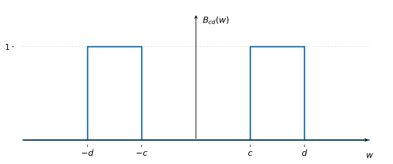
Fig. 4 Figure 1. The band-pass filter (“window”) \(B_{cd}(\omega)\), defined on the frequency axis \(\omega \in (-\infty,\, \infty)\). It equals \(1\) on the two symmetric frequency bands \([c,\, d]\) and \([-d,\, -c]\) and equals \(0\) everywhere else, with \(d > c > 0\).#
Define the time function
We have that \(y_{cd}(t)\), defined by
has the spectral density \(S_{cd}\) given by
If we choose an interval parameterized by \(0 < e < f\) such that \([e,\,f] \cap [c,\, d] = 0\), it follows from the orthogonal increments property of \(Z(\omega)\) that \(y_{ef}(t)\) is orthogonal to \(y_{cd}(t-\tau)\) for all \(t\). For using the Cramér representation, we have
since \(\overline{B_{ef}(\nu)}\ B_{cd}(\nu) = 0\) for all \(\nu\).
We also have that \(y_{ef}(t)\) has spectral density
By filtering the process \(x(t)\) with filters formed by taking disjoint frequency intervals, \([c,\,d]\), \([e,\,f]\), we create processes that are orthogonal at all leads and lags, but whose respective spectral densities equal that of \(x(t)\) over the intervals \([c,\,d]\) and \([e,\,f]\).
To motivate from another angle the frequency decomposition induced by the spectral density, it is useful to note that the Cramér representation
can be also represented in a couple of alternative ways. Let the complex valued random process \(Z'(\omega)\) be represented in the alternative forms
Then it is straightforward to derive the Cramér representation in the forms
where
and
where
The factor \(\sqrt{2/\pi}\) arises because the conjugate symmetry (ii) makes the negative frequencies duplicate the positive ones: \(x(t) = (2/\sqrt{2\pi})\,\operatorname{Re} \int_0^\infty e^{i\omega t} Z'(\omega)\, d\omega\), and \(2/\sqrt{2\pi} = \sqrt{2/\pi}\).
Representation (54) expresses \(x(t)\) as a weighted sum of cosine and sine waves, with the weights being random processes \(a(\omega)\) and \(b(\omega)\). Equation (55) represents \(x(t)\) as a sum of cosine waves with amplitude \(r(\omega)\) and phase \(\theta(\omega)\) being governed by random processes.
Using representation (54), it is possible to show that
the last equality using \(S(\omega) = S(-\omega)\). Formally \(E\,[a(\omega)^2 + b(\omega)^2] = E\,|Z'(\omega)|^2 = S(\omega)\,\delta(0)\), so the “random amplitudes” \(a(\omega),\ b(\omega)\) are, like \(Z'\) itself, generalized processes: the statement that has ordinary meaning is the one about increments, namely that the variance contributed by the frequency band \([c,\, d]\) is \(\frac{1}{\pi}\int_c^d S(\omega)\, d\omega\), which is what the band-pass construction above computed.
The time average as a filter: mean square ergodicity#
The machinery just assembled settles a question raised in 1. Covariance Stationary Stochastic Processes and left open there: when does averaging a single realization over time reveal the ensemble mean? The answer costs nothing extra, because the time average is simply one more filter of the kind (53) describes.
Let \(x(t)\) be covariance stationary with mean \(\mu\), and form the time average over a record of length \(2T\),
Call \(x(t)\) mean square ergodic if \(E(\bar x_T - \mu)^2 \to 0\) as \(T \to \infty\), so that \(\bar x_T\) converges in mean square to \(\mu\).
Now observe that \(\bar x_T\) is the output of a filter applied to \(x\), with weighting function \(b(\tau) = 1/2T\) on \([-T,T]\) and zero elsewhere. Its transfer function is
so by (52) the centered time average has the Cramér representation \(\bar x_T - \mu = (2\pi)^{-1/2}\int B_T(\omega) Z'(\omega)\, d\omega\), and by (53) its variance is
Equation (56) answers the question by inspection. The kernel \((\sin \omega T/\omega T)^2\) never exceeds \(1\), equals \(1\) at \(\omega = 0\), and tends to \(0\) at every \(\omega \neq 0\) as \(T\) grows. So as the record lengthens, the filter annihilates every frequency except the origin: time averaging is a band-pass filter whose band collapses onto zero frequency. What survives in the limit is whatever variance the process carries exactly at \(\omega = 0\).
For processes with an ordinary spectral density that limit is zero, and \(x\) is mean square ergodic. But the linearly deterministic component of Wold’s theorem (8. Spectral Densities) carries \(\delta\)-functions, \(S_d(\omega) = \sum_j a_j\pi[\delta(\omega - \omega_j) + \delta(\omega + \omega_j)]\), and if one of the \(\omega_j\) is zero then (56) retains a term that never vanishes. Hence
Criterion 3 (Mean square ergodicity)
A covariance stationary process is mean square ergodic if and only if its spectral density carries no \(\delta\)-function at frequency zero, equivalently iff its linearly deterministic component contains no zero-frequency term.
Failure has exactly one form: a random constant. If \(x(t) \equiv A\) with \(EA = 0\) and \(EA^2 = \sigma^2\), then \(R(\tau) = \sigma^2\) for every \(\tau\), the spectral density is \(2\pi\sigma^2\delta(\omega)\), and \(\bar x_T = A\) for every \(T\). The time average never approaches the ensemble mean, because there is nothing to average. Every purely linearly indeterministic process is therefore mean square ergodic, since its spectral density \(|\tilde P(i\omega)|^2\) is an ordinary function with no atoms. The book’s standing assumption already delivers the property.
Two consequences follow. First, when \(\int |R(\tau)|\,d\tau < \infty\), letting \(T \to \infty\) in the time-domain counterpart of (56),
gives
The variance of the sample mean is asymptotically \(S(0)/2T\): the spectral density at the origin, divided by the length of the record. The “long-run variance” of time series econometrics is nothing but the spectrum at zero frequency.
Second, and less comfortably: this settles the sample mean only. Whether the sample autocovariances converge to \(R(\tau)\) is a question about fourth moments. That is the property on which the estimation in 21. Inferring a Continuous-Time System from Discrete-Time Data: An Appreciation of A. W. Phillips (1959) and 22. The Dimensionality of the Aliasing Problem in Models with Rational Spectral Densities relies, which the second-moment theory of this book does not settle. A1. Ergodicity and the Consistent Estimation of Second Moments takes that up.
The band decomposition and sampling#
This chapter exhibits a process as a superposition of mutually orthogonal frequency bands, each carrying a definite share of the variance. Keep that picture in mind when reading 17. Discrete Sampling: The Folding Formula. Sampling at interval \(T\) does not destroy the bands; it wraps them. Every band is translated by a multiple of \(2\pi/T\) onto the observable interval \([-\pi/T,\, \pi/T]\) and there added to whatever was already present, which is precisely what the folding formula asserts. Because the bands were orthogonal to begin with, their variances simply add, and the discrete spectrum at a given frequency is the total variance of all the continuous bands that fold onto it. Nothing tells the observer how that total was divided among them.
That last sentence is the aliasing problem, and 22. The Dimensionality of the Aliasing Problem in Models with Rational Spectral Densities turns it into a construction: given any continuous spectral density, one can build a different one, supported entirely on high-frequency bands, that folds onto the same discrete spectrum. The alternative process is manufactured with exactly the band-pass window \(B_{cd}(\omega)\) of this chapter, applied at frequencies above the Nyquist rate. Two processes that could hardly look less alike in continuous time, one concentrated at low frequencies and the other carrying all of its power above \(\pi\), are then indistinguishable in the sampled data.
Exercises#
import numpy as np
from scipy.integrate import quad
Exercise 11
Variance by frequency band, and what sampling does to it. Take the Ornstein–Uhlenbeck process of 7. Stochastic Differential Equations Driven by a Wiener Process with \(a = 1\), \(b = 0.7\), whose spectral density is \(S(\omega) = b^2/(a^2+\omega^2)\).
(a) Verify that the band variances add up: partition \([0,\infty)\) into bands and check that \(\sum_{\text{bands}} \frac{1}{\pi}\int_c^d S(\omega)\, d\omega = R(0) = b^2/(2a)\), which is property (iii) of 8. Spectral Densities.
(b) Report the share of the variance lying above the Nyquist frequency \(\pi/T\) for \(T = 0.5\), \(1\) and \(3\). This is the power that sampling at interval \(T\) folds back into the observable band rather than discarding. That quantity governs how badly the formula of 17. Discrete Sampling: The Folding Formula distorts the spectrum.
(c) Confirm the orthogonality claim of the text numerically in the frequency domain: for disjoint bands, \(\int B_{cd}(\omega)\,B_{ef}(\omega)\,S(\omega)\,d\omega = 0\), so the band-pass filtered series are uncorrelated at all leads and lags.
Solution to Exercise 11
a, b = 1.0, 0.7
S = lambda w: b**2/(a**2 + w**2)
band_var = lambda c, d: quad(S, c, d, limit=200)[0]/np.pi     # variance in [c,d] and [-d,-c]

edges = [0, 0.5, 1, 2, 4, 8, 16, np.inf]
tot = 0.0
print("   band            variance     share")
for c, d in zip(edges[:-1], edges[1:]):
    v = band_var(c, d); tot += v
    print(f"  [{c:5.1f},{d:6.1f}]   {v:10.6f}   {v/(b**2/(2*a)):7.3%}")
print(f"\n  total = {tot:.8f},   R(0) = b^2/2a = {b**2/(2*a):.8f}")
   band            variance     share
  [  0.0,   0.5]     0.072316   29.517%
  [  0.5,   1.0]     0.050184   20.483%
  [  1.0,   2.0]     0.050184   20.483%
  [  2.0,   4.0]     0.034106   13.921%
  [  4.0,   8.0]     0.018814    7.679%
  [  8.0,  16.0]     0.009660    3.943%
  [ 16.0,   inf]     0.009736    3.974%

  total = 0.24500000,   R(0) = b^2/2a = 0.24500000
# (b) share of variance above the Nyquist frequency pi/T
for T in [0.5, 1.0, 3.0]:
    nyq = np.pi/T
    print(f"T={T:4.1f}:  Nyquist = {nyq:5.3f},  share of variance above it = "
          f"{band_var(nyq, np.inf)/(b**2/(2*a)):6.2%}")
T= 0.5:  Nyquist = 6.283,  share of variance above it = 10.05%
T= 1.0:  Nyquist = 3.142,  share of variance above it = 19.62%
T= 3.0:  Nyquist = 1.047,  share of variance above it = 48.53%
# (c) disjoint bands are orthogonal
B = lambda w, c, d: 1.0 if c <= w <= d else 0.0
cross = quad(lambda w: B(w,0.5,1.0)*B(w,2.0,4.0)*S(w), 0, 8, limit=400)[0]
print(f"cross term for disjoint bands [0.5,1] and [2,4]: {cross:.3e}")
cross term for disjoint bands [0.5,1] and [2,4]: 0.000e+00
The band variances sum to \(R(0)\), and disjoint bands contribute nothing to each other. Part (b) is the quantitative form of the warning in 17. Discrete Sampling: The Folding Formula: at \(T = 0.5\) about a tenth of the variance sits above the Nyquist frequency, so the folded spectrum departs from the continuous one only modestly; by \(T = 3\) nearly half of it does, and the discrete spectrum is visibly inflated. The share falls slowly. The Lorentzian tail decays only as \(\omega^{-2}\), so halving the sampling interval does not come close to halving the aliased power. 22. The Dimensionality of the Aliasing Problem in Models with Rational Spectral Densities pushes this to its extreme by building a process whose variance lies entirely above the Nyquist frequency, yet which is indistinguishable from this one in sampled data.
Exercise 12
Mean square ergodicity, and how it fails. Continue with the Ornstein–Uhlenbeck process, \(R(\tau) = \frac{b^2}{2a}e^{-a|\tau|}\), \(S(\omega) = b^2/(a^2+\omega^2)\), \(a=1\), \(b=0.7\).
(a) Evaluate \(E(\bar x_T-\mu)^2\) from the time-domain formula \(\frac{1}{2T}\int_{-2T}^{2T}(1-|\tau|/2T)R(\tau)d\tau\) for \(T = 5, 20, 100\), and confirm it approaches \(S(0)/2T\) of (57).
(b) Confirm the same numbers from the frequency-domain formula (56), integrating \((\sin\omega T/\omega T)^2 S(\omega)\). The two routes are the same computation seen from the two sides of the Cramér representation.
(c) Now break ergodicity. Add a random constant: \(y(t) = x(t) + A\) with \(A\) independent of \(x\), mean zero, variance \(\sigma^2 = 0.5\). Show that \(E(\bar y_T - \mu)^2 \to \sigma^2\) rather than to zero, however long the record. The spectral density of \(y\) carries a \(\delta\)-function at \(\omega = 0\).
Solution to Exercise 12
import numpy as np
from scipy.integrate import quad

a, b = 1.0, 0.7
R = lambda t: (b**2/(2*a))*np.exp(-a*abs(t))
S = lambda w: b**2/(a**2 + w**2)
S0 = b**2/a**2                                   # = S(0) = integral of R

print("  T      time domain      S(0)/2T       frequency domain")
for T in [5.0, 20.0, 100.0]:
    td = quad(lambda t: (1-abs(t)/(2*T))*R(t), -2*T, 2*T, limit=400)[0]/(2*T)
    fd = quad(lambda w: (np.sin(w*T)/(w*T))**2 * S(w), -np.inf, np.inf, limit=800)[0]/(2*np.pi)
    print(f"{T:6.1f}   {td:.8f}     {S0/(2*T):.8f}    {fd:.8f}")
  T      time domain      S(0)/2T       frequency domain
   5.0   0.04410022     0.04900000    0.04410022
  20.0   0.01194375     0.01225000    0.01194375
 100.0   0.00243775     0.00245000    0.00243775
# (c) a random constant added: variance of the sample mean no longer vanishes
sig2 = 0.5
print("  T      Var(mean of y) = Var(mean of x) + sigma^2")
for T in [5.0, 20.0, 100.0, 1000.0]:
    td = quad(lambda t: (1-abs(t)/(2*T))*R(t), -2*T, 2*T, limit=400)[0]/(2*T)
    print(f"{T:7.1f}   {td + sig2:.8f}   -> floor of sigma^2 = {sig2}")
  T      Var(mean of y) = Var(mean of x) + sigma^2
    5.0   0.54410022   -> floor of sigma^2 = 0.5
   20.0   0.51194375   -> floor of sigma^2 = 0.5
  100.0   0.50243775   -> floor of sigma^2 = 0.5
 1000.0   0.50024488   -> floor of sigma^2 = 0.5
The time-domain and frequency-domain evaluations agree to eight digits, and both approach \(S(0)/2T\). Adding the random constant puts an atom at the origin, and the variance of the sample mean falls to \(\sigma^2\) and stops: no record, however long, locates \(\mu\). Note that \(A\) is invisible in any centered second moment. It shifts \(R(\tau)\) by \(\sigma^2\) at every lag, which the sample autocovariances of a demeaned record cannot detect.