6. The Wiener Process

We shall now describe a class of stochastic processes that can be described by stochastic differential equations driven by a “Wiener Process.” We shall approach the Wiener process by regarding it as the limit as \(\lambda \to \infty\) of a process \(x(t)\) that solves

(28)\[ dx(t) = 1/\sqrt\lambda\, \left(dN_1(t) - dN_2(t)\right) \]

where \(N_1\) and \(N_2\) are independent Poisson counters with rates \(\lambda/2\). We have already seen that for \(\lambda > 0\), this process is a random walk with jumps of size \(\pm\, 1/\sqrt\lambda\) occurring at times that arrive at a mean rate of \(\lambda/2\) per unit of time. As we drive \(\lambda\) toward infinity, the jump size \(1/\sqrt\lambda\) goes to zero, while the average number of arrivals or jumps per unit of time goes to infinity. We have seen that the mean function and autocorrelation function of the solution \(x(t)\) of (28) are given by

\[\begin{split} \begin{aligned} E x(t) &= 0 \\ R(t,\, t + \tau) &= \min\ (t,\, t + \tau) \end{aligned} \end{split}\]

and so are independent of \(\lambda\). These functions also characterize the process that results in the limit as \(\lambda \to \infty\). The sample paths of the limiting process are continuous with probability one but differentiable nowhere. Roughly speaking, the sample paths are continuous because the jumps in the process become infinitesimal as \(\lambda \to \infty\); the sample paths are differentiable nowhere because there are “so many” of these infinitesimal jumps in a small interval of time.

We begin by computing the \(p^{th}\) moments of the process governed by

\[ dx(t) =\ \frac{1}{\sqrt\lambda}\ \left(dN_1(t) - dN_2\,(t)\right) \]

where \(N_1\) and \(N_2\) are two independent Poisson counters with identical rates \(\lambda/2 > 0\). Using rule (20), we have that for \(p > 0\)

\[\begin{split} \begin{aligned} dx^p &= \left[(x + \frac{1}{\sqrt\lambda}\,)^p - x^p\right]\, dN_1 + \left[(x - \frac{1}{\sqrt\lambda})^p - x^p\right]\, dN_2 \\ &= \left( px^{p-1}\ \frac{1}{\sqrt\lambda}\ + \binom{p}{2}\, x^{p-2}\ \left(\frac{1}{\sqrt\lambda}\right)^2\ + \cdots + \left(\frac{1}{\sqrt\lambda}\right)^p\right)\, dN_1 \\ &+ \left( -px^{p-1}\ \frac{1}{\sqrt\lambda}\ + \binom{p}{2}\, x^{p-2}\ \left(\frac{1}{\sqrt\lambda}\right)^2 + \cdots \pm\, \left(\frac{1}{\sqrt\lambda}\right)^p\right)\, dN_2. \end{aligned} \end{split}\]

It follows from rule (23) that

(29)\[\begin{split} \begin{aligned} \frac{d}{dt}\ E x^p &= \binom{p}{2}\ \left(\frac{1}{\lambda}\right)\ E x^{p-2}\, \lambda + \binom{p}{4}\ \left(\frac{1}{\lambda}\right)^2\ E x^{p-4}\, \lambda + \cdots + \left(\frac{1}{\sqrt\lambda}\right)^{p}\, \lambda \\ p\ &\text{ even, }\ p \geq 2 \end{aligned} \end{split}\]

(30)\[\begin{split} \begin{aligned} \frac{d}{dt}\ E x^p &= \binom{p}{2}\ \left(\frac{1}{\lambda}\right)\ E x^{p-2}\, \lambda + \binom{p}{4}\ \left(\frac{1}{\lambda}\right)^2\, E x^{p-4}\, \cdot\, \lambda + \ldots + \binom{p}{p-1} \left(\frac{1}{\sqrt\lambda}\right)^{p-1}\ E x \cdot \lambda \\ &\ p\ \text{ odd} \end{aligned} \end{split}\]

We have calculated that \(E x(t) = 0\), and that \(E x(t)^2 = t\). Using (30) recursively to calculate odd moments, we find that

\[ E x(t)^p = 0\ \text{ for }\ p\ \text{ odd.} \]

For even powers of \(p\) higher than 2, we drive \(\lambda \to \infty\) in (29) and find that

\[ \frac{d}{dt}\ E x^p = \binom{p}{2}\, E x^{p-2}, \]

which has the solution

\[ E x^p = \frac{1}{2}\, \int_0^t p\, (p-1)\ E x^{p-2}\, (s)ds. \]

Using this equation recursively, starting from \(p = 2\) gives

(31)\[\begin{split} \begin{aligned} E x(t)^2 &= t \\ E x(t)^4 &= \frac{1}{2} \int_0^t 4 \cdot 3 \cdot sds = 3 t^2 \\ E x(t)^6 &= 15 t^3 \end{aligned} \end{split}\]

and so on.

Now for the Gaussian density function

\[ f(x) = (2 \pi \sigma^2)^{-1/2}\ \exp\ \frac{-x^2}{2 \sigma^2}\, , \]

with variance \(\sigma^2\), integration by parts shows that \(E x^p = 0\) for \(p\) odd, while for \(p\) even

(32)\[ E x^p = \sigma^{p}\ (p - 1)\ (p - 3)\ \ldots\ 1.\ p\ \text{ even} \]

It is known that if all of the moments of a process equal those of a Gaussian process, then that process is itself Gaussian. Comparing (31) with (32), we can conclude that the limiting process as \(\lambda \to \infty\) is Gaussian with mean zero and variance \(t\). That is, \(x(t)\) has density

\[ f\left(x(t)\right) = (2 \pi t)^{-1/2}\ \exp\ \frac{-x(t)^2}{2 t}\, ,\ t \geq 0. \]

We shall denote the limiting process as \(\lambda \to \infty\) as \(W(t)\). It is known as Brownian motion or a Wiener process.

The Wiener process \(W(t)\) is characterized by the following properties.

(i) \(W(0) = 0\)

(ii) \(W(t_1) - W(t_2)\) and \(W(t_3) - W(t_4)\) are independent if \([t_1,\, t_2]\) and \([t_3,\, t_4]\) are disjoint intervals.

(iii) \(E(W(t) - W(\tau))^2 = |t - \tau|\).

(iv) Sample paths or realizations of \(W(t)\) are continuous with probability 1.

Property (ii) is the independent increments property, and is inherited from the Poisson process of which \(W(t)\) is the limit. 7. Stochastic Differential Equations Driven by a Wiener Process studies stochastic differential equations driven by this \(W(t)\) and states Itô’s rule for manipulating them.

Exercises

import numpy as np
import matplotlib.pyplot as plt

Exercise 4

The text builds the Wiener process as the limit \(\lambda \to \infty\) of

\[ dx(t) = \frac{1}{\sqrt{\lambda}}\,\bigl(dN_1(t) - dN_2(t)\bigr), \]

where \(N_1, N_2\) are independent Poisson counters of rate \(\lambda/2\). The value at \(t = 1\) is \(x(1) = \lambda^{-1/2}\bigl(N_1(1) - N_2(1)\bigr)\), where \(N_1(1), N_2(1)\) are independent \(\operatorname{Poisson}(\lambda/2)\) variables.

Draw many samples of \(x(1)\) for \(\lambda \in \{4, 40, 400\}\) and show that the histogram of \(x(1)\) converges to the standard normal density (mean \(0\), variance \(1\)) as \(\lambda\) grows, illustrating that the limiting process is Gaussian with \(E\,x(1)^2 = 1\).

Solution to Exercise 4

rng = np.random.default_rng(7)
g = np.linspace(-4, 4, 200)
std_normal = np.exp(-g**2 / 2) / np.sqrt(2 * np.pi)

fig, axes = plt.subplots(1, 3, figsize=(13, 4), sharey=True)
for ax, lam in zip(axes, [4, 40, 400]):
    N1 = rng.poisson(lam / 2, size=200_000)
    N2 = rng.poisson(lam / 2, size=200_000)
    x1 = (N1 - N2) / np.sqrt(lam)              # x(1) for this lambda
    ax.hist(x1, bins=80, density=True, alpha=0.6)
    ax.plot(g, std_normal, 'r-', lw=2)
    ax.set_title(rf'$\lambda={lam}$,  var $={x1.var():.2f}$')
    ax.set_xlabel('$x(1)$')
axes[0].set_ylabel('density')
plt.show()

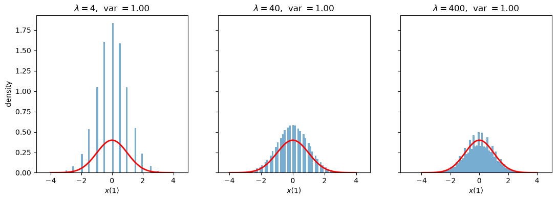
For small \(\lambda\) the distribution of \(x(1)\) is visibly discrete (jumps of size \(\lambda^{-1/2}\)), but as \(\lambda\) grows the jumps shrink and the distribution fills in the standard normal bell curve, with variance approaching \(1\).

Exercise 5

Once the Wiener process is in hand it is most convenient to simulate it directly from its Gaussian independent increments: on a grid of spacing \(dt\), the increments \(W(t+dt) - W(t)\) are i.i.d. \(\mathcal{N}(0, dt)\), so \(W\) is a cumulative sum of such increments.

(a) Using this construction, verify the even-moment formulas derived in the text, \(E\,W(1)^2 = 1\), \(E\,W(1)^4 = 3\), and \(E\,W(1)^6 = 15\).

(b) Verify that the quadratic variation \(\sum_k \bigl(W(t_{k+1}) - W(t_k)\bigr)^2\) over \([0, 1]\) concentrates at \(1\) as the mesh shrinks. A process that is continuous but of unbounded variation behaves this way, and this is the source of the extra term in Itô’s rule (Chapter 7).

Solution to Exercise 5

rng = np.random.default_rng(11)
n, dt = 40_000, 0.002
steps = int(1.0 / dt)

dW = rng.normal(0.0, np.sqrt(dt), size=(n, steps))   # Gaussian increments
W = np.cumsum(dW, axis=1)
WT = W[:, -1]                                         # W(1) across paths

# (a) even moments of W(1)
for p, theory in [(2, 1), (4, 3), (6, 15)]:
    print(f"E[W(1)^{p}] = {np.mean(WT**p):6.3f}   (theory {theory})")

E[W(1)^2] =  0.996   (theory 1)
E[W(1)^4] =  2.949   (theory 3)
E[W(1)^6] = 14.540   (theory 15)

# (b) quadratic variation on [0, 1]
qv = np.sum(dW**2, axis=1)
print(f"quadratic variation over [0,1]: mean {qv.mean():.4f},  std {qv.std():.4f}  (theory 1)")

quadratic variation over [0,1]: mean 1.0002,  std 0.0633  (theory 1)

The second and fourth moments match \(1\) and \(3\) closely; the sixth moment (\(15\)) carries more Monte Carlo error because it weights the tails heavily. The quadratic variation clusters tightly around \(1\) with a small standard deviation that would shrink further as \(dt \to 0\).