13. Locally Unpredictable Stochastic Processes#
Lack of mean square differentiability implies that a process is “locally unpredictable” or is “locally like a martingale.” Sims used the concept of local unpredictability in his work on asset prices, interest rates, and consumption.
This chapter is where the thread begun in 2. Mean Square Continuity and Differentiability of a Stochastic Process arrives at its economic payoff. There, mean square differentiability was tied to the existence of \(R''(0)\); in 9. Characterizations of Mean Square Differentiability and Mean Square Continuity that became the condition \(p(0) = 0\) on the Wold kernel; in 11. Linear Stochastic Differential Equations it became a count, \(n - 1 - m\), read off the degrees of two polynomials. Here the failure of that condition means something. Over short intervals, a process whose kernel does not vanish at the origin is unforecastable. We use the following definition:
Definition 10
A stochastic process \(x(t)\) with finite second moments is said to be locally unpredictable if
This definition makes precise the sense in which \(x(t)\) is locally a martingale, i.e., the sense in which for small \(\delta\),
We have the following theorem.
Theorem 16
Let \(x(t)\) be a linearly indeterministic covariance stationary stochastic process with Wold representation
where \(w(t)\) is a fundamental white noise for the \(x(t)\) process, and \(Ew(t) w(t-\tau) = \delta(\tau)\). Assume that \(p(\tau)\) is twice continuously differentiable, with \(p'\) and \(p''\) square integrable. Then if \(x(t)\) is not mean square differentiable, \(x(t)\) is locally unpredictable.
Proof. From the Wiener-Kolmogorov prediction formula, we have that
Taking the limit as \(\delta \to 0\) gives, after applying l’Hospital’s rule,
If \(p(0) \neq 0\), this limit is given by
Upon noting that \(p(0) = 0\) if and only if \(x(t)\) is mean square differentiable (by 9. Characterizations of Mean Square Differentiability and Mean Square Continuity: with \(p'\) square integrable, mean square differentiability reduces to the single condition \(p(0) = \lim_{s\to\infty} s\tilde P(s) = 0\)), we have the desired result that if \(x(t)\) is not mean square differentiable, then \(x(t)\) is locally unpredictable.
For the rational linear stochastic differential equations of 11. Linear Stochastic Differential Equations, this dividing line is explicit. There \(x(t)\) is mean square differentiable \(n - 1 - m\) times, where \(n\) and \(m\) are the degrees of the denominator operator \(\theta(D)\) and the numerator operator \(\psi(D)\); by the initial value theorem, \(p(0) = \lim_{s\to\infty} s\tilde P(s) \neq 0\) exactly when \(m = n - 1\). The locally unpredictable members of this family are therefore precisely those with \(n - 1 - m = 0\), a numerator just one degree below the denominator. Every smoother member, with \(m < n - 1\), is locally predictable.
Using the preceding theorem and our formula (70) for geometric distributed leads from 12. Linear Least Squares Prediction, it is straightforward to establish that if \(x(t)\) is a covariance stationary stochastic process with Wold representation
then for any \(\rho < 0\), the geometric sum of future expected \(x\)’s,
is locally unpredictable, even if \(x(t)\) is mean square differentiable. To show this, we apply the initial value theorem of 9. Characterizations of Mean Square Differentiability and Mean Square Continuity to the kernel \(g\):
(Here we are using that \(\lim_{s\to \infty} s\tilde P (s) = 0\) by the assumption of mean square differentiability of \(x(t)\).) We know that \(\tilde P (-\rho) \neq 0\) because \(\tilde P(s)\) has no zeroes in the right half plane, by the assumption that (72) is a Wold representation.
This last result carries the chapter’s economic content. Taking a present value manufactures local unpredictability. However smooth the dividend, income, or endowment process \(x\) may be, the asset price or permanent income built from it behaves, over short intervals, like a martingale. Nothing about tastes or market structure is needed for the conclusion; it follows from the algebra of the annihilation operator.
Exercises#
The ratio in Definition 10 can be computed for any kernel, at any \(\delta\), directly from the expression established in the proof:
The numerator is the variance of the \(\delta\)-ahead forecast error; the denominator is the variance of the actual change \(x(t+\delta) - x(t)\). A process is locally unpredictable when the forecast error accounts for all of the movement in the limit.
import numpy as np
import matplotlib.pyplot as plt
from scipy.integrate import quad

def varrho(p, delta, upper=60.0):
    """The local-unpredictability ratio at horizon delta, for a one-sided kernel p."""
    num, _ = quad(lambda s: p(s)**2, 0.0, delta, limit=200)
    rev, _ = quad(lambda s: (p(s + delta) - p(s))**2, 0.0, upper, limit=400)
    return num / (num + rev)
Exercise 15
The dividing line. Take \(a = 1\) and compare two kernels from the rational family of 11. Linear Stochastic Differential Equations:
The first has \(p_1(0) = 1 \neq 0\) and is differentiable \(n-1-m = 0\) times; the second has \(p_2(0) = 0\) and is differentiable once.
(a) Compute \(\varrho(\delta)\) for each over a range of \(\delta\) and verify that \(\varrho \to 1\) for \(p_1\) and \(\varrho \to 0\) for \(p_2\).
(b) Explain the rates. Show analytically that for a kernel with \(p(0)\neq 0\) the numerator of (73) is \(O(\delta)\) while the second term of the denominator is \(O(\delta^2)\), whereas for a kernel with \(p(0)=0\) they are \(O(\delta^3)\) and \(O(\delta^2)\) respectively. Hence \(\varrho(\delta) \to 1\) in the first case and \(\varrho(\delta) = O(\delta)\to 0\) in the second.
Solution to Exercise 15
(b) If \(p(0) \neq 0\) then \(p(s)^2 \approx p(0)^2\) near the origin, so \(\int_0^\delta p^2 \approx p(0)^2\delta\). Meanwhile \(p(s+\delta)-p(s)\approx \delta p'(s)\), so the revision term is \(\approx \delta^2\int_0^\infty p'^2\). The ratio is \(p(0)^2\delta / [p(0)^2\delta + O(\delta^2)] \to 1\). If instead \(p(0)=0\) then \(p(s)\approx p'(0)s\) near the origin and \(\int_0^\delta p^2 \approx p'(0)^2\delta^3/3\), while the revision term is still \(O(\delta^2)\); the ratio is therefore \(O(\delta) \to 0\). The whole distinction is the behaviour of \(p\) at the origin.
a = 1.0
p1 = lambda s: np.exp(-a*s)          # p(0) = 1  -> locally unpredictable
p2 = lambda s: s*np.exp(-a*s)        # p(0) = 0  -> mean square differentiable

deltas = np.logspace(-3, 0.3, 40)
r1 = np.array([varrho(p1, d) for d in deltas])
r2 = np.array([varrho(p2, d) for d in deltas])

for d, x, y in zip(deltas[::13], r1[::13], r2[::13]):
    print(f"delta={d:7.4f}   varrho(p1)={x:.4f}   varrho(p2)={y:.4f}")
delta= 0.0010   varrho(p1)=0.9995   varrho(p2)=0.0013
delta= 0.0126   varrho(p1)=0.9937   varrho(p2)=0.0166
delta= 0.1585   varrho(p1)=0.9267   varrho(p2)=0.1854
delta= 1.9953   varrho(p1)=0.5680   varrho(p2)=0.6415
wide = np.logspace(-3, 1.2, 60)
R1 = np.array([varrho(p1, d, upper=200.0) for d in wide])
R2 = np.array([varrho(p2, d, upper=200.0) for d in wide])

fig, ax = plt.subplots(figsize=(9, 5))
ax.semilogx(wide, R1, 'o-', lw=2, ms=4, label=r'$p(\tau)=e^{-a\tau}$,  $p(0)\neq 0$')
ax.semilogx(wide, R2, 's-', lw=2, ms=4, label=r'$p(\tau)=\tau e^{-a\tau}$,  $p(0)=0$')
ax.axhline(1, color='0.6', ls=':')
ax.axhline(0, color='0.6', ls=':')
ax.axhline(0.5, color='0.4', ls='--', lw=1,
           label=r'$\varrho \to 1/2$ as $\delta\to\infty$ (any stationary process)')
ax.set_xlabel(r'forecast horizon $\delta$  (log scale)')
ax.set_ylabel(r'local-unpredictability ratio $\varrho(\delta)$')
ax.set_title('Local unpredictability is decided by the kernel at the origin')
ax.legend(fontsize=9); plt.show()
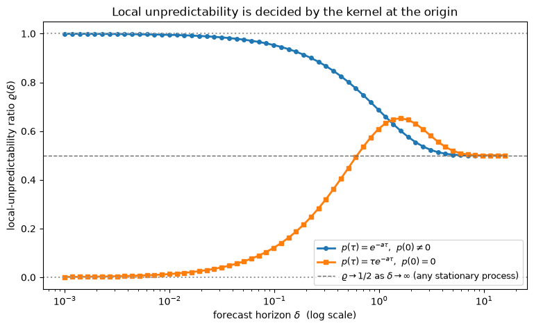
The figure shows why the limit at zero is the thing to look at. At long horizons the two curves are indistinguishable: both tend to \(\tfrac12\), as they must for any stationary process, since the forecast error variance tends to \(R(0)\) while \(E(x(t+\delta)-x(t))^2 \to 2R(0)\). It is only as \(\delta \to 0\) that the processes separate, and then they separate completely. For \(p_1\) nearly all of the movement over \([t, t+\delta]\) is unforecastable; for \(p_2\) nearly none of it is. The two kernels differ only by a factor of \(\tau\); that is, only in their behaviour at the origin.
Exercise 16
Present values are locally unpredictable. Let \(x\) have the smooth kernel \(p(\tau) = \tau e^{-a\tau}\) of the previous exercise, so that \(x\) is mean square differentiable and, by Exercise 15, locally predictable. Form the present value
(a) Show that the kernel of \(x^*\) is \(g(s) = \int_0^\infty e^{\rho u}\, p(s+u)\, du\), and that for this \(p\),
(b) Verify numerically that \(\varrho(\delta) \to 1\) for \(g\), so that \(x^*\) is locally unpredictable even though \(x\) is not. Interpret: if \(x\) is a dividend and \(x^*\) a stock price, a smooth dividend process delivers a price that behaves locally like a martingale.
Solution to Exercise 16
(a) Writing \(x(t+s) = \int_0^\infty p(\tau)w(t+s-\tau)d\tau\) and keeping only the terms dated \(t\) or earlier, \(E_t x(t+s) = \int_0^\infty p(\tau+s) w(t-\tau)d\tau\). Multiplying by \(e^{\rho s}\) and integrating over \(s\) gives \(x^* = \int_0^\infty g(\tau)w(t-\tau)d\tau\) with \(g\) as stated. For \(p(\tau)=\tau e^{-a\tau}\), \(g(s) = e^{-as}\int_0^\infty (s+u)e^{-(a-\rho)u}du\), which integrates to the displayed form. Setting \(s=0\) gives \(g(0) = (a-\rho)^{-2}\), and \(\tilde P(s) = (s+a)^{-2}\) evaluated at \(-\rho\) is the same thing, confirming \(g(0) = \tilde P(-\rho)\) of the text.
rho = -0.5
g  = lambda s: np.exp(-a*s)*(s/(a-rho) + 1/(a-rho)**2)

# check (a): the closed form against the defining integral, and against P(-rho)
for s in [0.0, 0.7, 2.0]:
    direct, _ = quad(lambda u: np.exp(rho*u)*p2(s+u), 0, 80, limit=300)
    print(f"s={s:4.1f}:  g(s) closed form = {g(s):.8f},  integral = {direct:.8f}")
print(f"g(0) = {g(0.0):.8f},  P(-rho) = 1/(a-rho)^2 = {1/(a-rho)**2:.8f}")
s= 0.0:  g(s) closed form = 0.44444444,  integral = 0.44444444
s= 0.7:  g(s) closed form = 0.45244439,  integral = 0.45244439
s= 2.0:  g(s) closed form = 0.24059606,  integral = 0.24059606
g(0) = 0.44444444,  P(-rho) = 1/(a-rho)^2 = 0.44444444
rg = np.array([varrho(g, d) for d in deltas])

fig, ax = plt.subplots(figsize=(9, 5))
ax.semilogx(deltas, r2, 's-', lw=2, color='C1',
            label=r'$x$: kernel $\tau e^{-a\tau}$  (smooth, locally predictable)')
ax.semilogx(deltas, rg, 'D-', lw=2, color='C3',
            label=r'$x^*=E_t\int e^{\rho s}x(t+s)ds$  (locally unpredictable)')
ax.axhline(1, color='0.6', ls=':'); ax.axhline(0, color='0.6', ls=':')
ax.set_xlabel(r'forecast horizon $\delta$  (log scale)')
ax.set_ylabel(r'$\varrho(\delta)$')
ax.set_title('Taking a present value manufactures local unpredictability')
ax.legend(fontsize=9); plt.show()
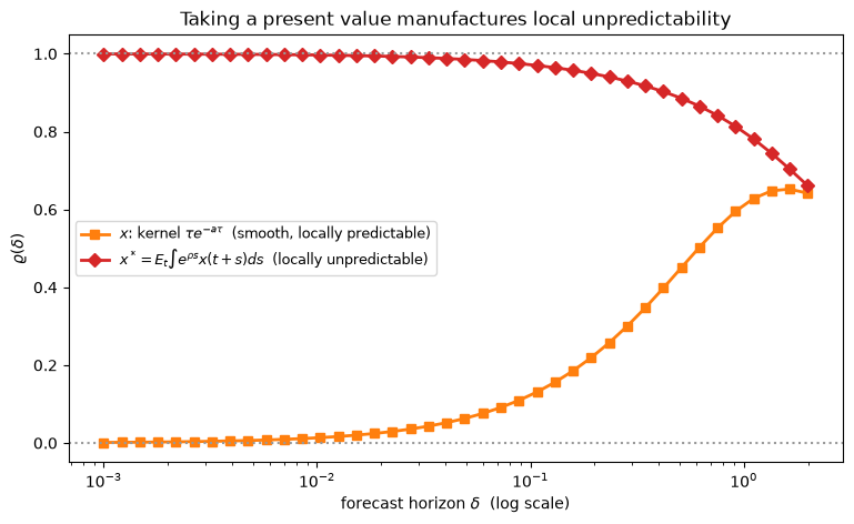
The present-value operator moves the process across the dividing line. The reason is visible in the closed form for \(g\): the operator adds a constant term \((a-\rho)^{-2}\) to a kernel that previously vanished at the origin. This is the formal content of the observation, due to Sims and to Hall, that asset prices and consumption should look like martingales at high frequency even when the fundamentals driving them are smooth. 18. Time Aggregation finds for that reason that the sampling distortions of Table 1 are less severe for present-value variables than for the smooth processes underlying them.