20. Aggregation Over Time and the Inverse Optimal Predictor Problem for Adaptive Expectations in Continuous Time#
Note
This chapter reports and paraphrases the analysis of Lars Peter Hansen and Thomas J. Sargent, “Aggregation Over Time and the Inverse Optimal Predictor Problem for Adaptive Expectations in Continuous Time,” International Economic Review 24 (1983), no. 1, pp. 1–20. We retell the argument in the third person, writing “Hansen and Sargent show” and “the authors now assume,” and we preserve the original section, equation, and table numbering. We recompute the four tables of the original paper in Python, and the code adds figures that are not in the original. The recomputation reproduces the published tables to all printed digits, except for three entries of Table 2 that are typographical errors in the 1983 original. 5. Predicting inflation using information on lagged inflation and lagged money creation flags them.
1. Introduction#
In 1956 Milton Friedman (1957) and Phillip Cagan (1956) formulated and applied the adaptive expectations hypothesis. Shortly thereafter, John F. Muth (1960) solved the following “inverse optimal predictor” problem: for what discrete-time, univariate stochastic process is the discrete-time version of the adaptive expectations mechanism optimal in the sense of delivering linear least squares forecasts? Much later Sargent (1977) solved the following extended inverse optimal predictor problem: in the context of a discrete-time version of Cagan’s model of portfolio balance, for what bivariate money creation, inflation stochastic process does a discrete-time version of adaptive expectations deliver linear least squares forecasts for inflation?
Hansen and Sargent solve the continuous-time version of both of these inverse optimal predictor problems. The continuous-time adaptive expectations scheme itself was derived as an optimal forecast in 14. Examples of Nonstationary Processes (equation (81) there); this chapter takes that scheme as its starting point and asks what aggregation over time does to it. In the context of a continuous-time version of Cagan’s portfolio schedule, they find the continuous-time, generalized stochastic process for the money supply and price level that makes the adaptive expectations mechanism yield linear least squares forecasts for inflation. The problem is of interest if only because Cagan himself formulated his model in continuous time, as have many others, even though he ultimately estimated an approximating discrete-time model. To pin down the “optimal” discrete-time approximating model, the authors deduce the discrete-time process for point-in-time observations on the money supply and price level implied by the continuous-time model that makes adaptive expectations rational. This makes precise a sense in which the discrete-time adaptive expectations scheme approximates a model in which agents form adaptive expectations optimally in continuous time. Hansen and Sargent also derive an exact formula linking the discrete-time adaptive expectations decay parameter \(\lambda\) to the continuous-time decay parameter \(\beta\), and compare it to the approximation \(\lambda = \exp(-\beta)\) used by Cagan.
The continuous-time process for inflation and money creation that makes adaptive expectations optimal has, ipso facto, the property that money creation fails to Granger (1969) cause inflation in continuous time. Yet for discrete-time samples drawn from that same process, money creation does Granger cause inflation. This is an instance of how aggregation over time interrupts Granger non-causality patterns that hold in continuous time. Sims (1971, 1973) studied that phenomenon, 18. Time Aggregation takes it up systematically, and the spectral folding of 17. Discrete Sampling: The Folding Formula is its root. The model is simple enough that Hansen and Sargent can analyze the effect quite completely.
The calculations are interesting for their own sake, and also because they illustrate a method for analyzing the effects of aggregation over time that applies to a wide variety of linear rational expectations models.
2. The continuous-time inverse optimal predictor problem#
Hansen and Sargent begin with Cagan’s portfolio balance schedule in continuous time
where \(p(t)\) is the logarithm of the price level, \(m(t)\) is the logarithm of the money supply, \(a(t)\) is a random disturbance to the portfolio balance schedule, \(D^{+}\) is the mean square right time derivative operator, and \(\hat E_t\) is the linear least squares projection operator onto an information set that includes at least current and past observations on \(p\), \(m\), and \(a\). The authors do not require that the \(p\) process be mean square differentiable, but only that \(\{\hat E_t\, p(t+v): v \geq 0\}\) be mean square differentiable for \(v > 0\) and have a mean square right derivative at \(v = 0\). This right derivative is denoted \(D^{+}\hat E_t\, p_t\).
To solve stochastic differential equation (167), Hansen and Sargent write it shifted ahead \(v\) time units as
Projecting both sides of (168) onto the \(t\) period information set gives
where \(D\) is the time derivative operator. The realizable, time invariant solution to (169) is just
where \(\rho = 1/\alpha < 0\). Taking limits as \(v\) declines to zero, and noting that \(\lim_{v \downarrow 0}\hat E_t\, p(t+v) = \hat E_t\, p(t) = p(t)\), one obtains
as the solution to (167). (Dividing (169) by \(\alpha\) puts it in the form \((D + \rho)\hat E_t p(t+v) = \rho\,[\hat E_t m(t+v) - \hat E_t a(t+v)]\); since \(\rho < 0\) the root \(-\rho\) lies in the right half plane, so the bounded solution is the forward one displayed above. As a check, if \(m\) and \(a\) are constant there is no expected inflation and (167) requires \(p = m - a\), which is what (170) delivers, since \(\rho\int_0^\infty e^{\rho u}\, du = -1\).)
Hansen and Sargent now specialize the assumptions so that Cagan’s adaptive expectations mechanism is optimal: they seek specifications for \(a\) and \(m\) that, together with (170), imply that
In expression (171) \(Dp\) is not necessarily required to be an ordinary stochastic process but rather can be a generalized stochastic process so long as the integral on the right-hand side is well defined. On the other hand, \(\{D\hat E_t\, p(t+v): v > 0\}\) is assumed to be an ordinary stochastic process. Thus, even though inflation itself may not be physically realizable, the authors assume that anticipated inflation is. Equation (171) also implies that at each instant inflation is expected to be constant over the entire future, since its right-hand side does not depend on \(v\).
The authors assume that the joint process \(x\) given by
has a time invariant Wold representation
In equation (172) \(c(D)\) is a one-sided matrix convolution operator and \(w\) is a continuous-time white noise vector with \(Ew(t) = 0\) and
where \(\delta\) is the Dirac delta generalized function. They assume that (172) holds for some \(t\) greater than or equal to a start-up time \(T\), with \(w(t) = 0\) for \(t < T\). That (172) is a Wold representation means that instantaneous forecast errors in predicting an element of \(x(t)\) from past \(x\)’s are linear combinations of the elements of \(w(t)\).
Hansen and Sargent write the first row of (172) as
The operator that shifts a time subscript \(v\) units ahead can be represented as \(e^{vD}\). Shifting (173) forward \(v\) time units and taking expectations, they find
where \([\ ]_+\) is the annihilation operator that instructs one to ignore portions of the convolution operator that are concentrated on the negative numbers. Equation (171) implies that
for all \(v > 0\). It is verified in the appendix that the solution to this operator equation is
where \(k_0\) is an arbitrary row vector of constants. The authors are free to normalize \(c\) and \(w\) so that
where \(w_1\) is the first element of \(w\) and \(k_1\) is an arbitrary scalar constant. Specification (174) implies that
as one verifies by evaluating the annihilation operator of the appendix: with \(c_1(D) = (D+\beta)k_1/D^2\),
Substituting (175) into equation (167) shows that
Equation (176) is a version of Cagan’s model in continuous time, since
which is the right-hand side of the adaptive expectations scheme (171).
Equation (176) reveals an exact relationship among \(m\), \(p\), and \(a\). This singularity means that the white noise vector \(w\) can have at most two elements. The authors assume that the \(x\) process has maximal rank, so that \(w\) has exactly two elements. Partitioning \(w\) and \(c\), they write
where
Substituting (177) into equation (167) and equating coefficients on \(w_1(t)\) and \(w_2(t)\) shows that
The stochastic process \(a\) is assumed not to be observed by the econometrician. To give equation (167) empirical content, something must be said about the dynamic correlation between \(a\) and \(m\). Hansen and Sargent require that, for \(v > 0\),
Assumption (179) says that no other variables observed by private agents Granger cause (help predict) \(a\). It implies that
for some scalar constant \(k_2\). Combining restrictions (180) and (178) determines that
Restriction (181) is a restriction on the bivariate moving average representation for the observable process
\alpha \beta k_1 + k_1 + k_2 k_3 = 0. $$
In this case
and the moving average representation for \(p\) and \(m\) is
In the continuous-time system (182), \(m\) fails to Granger cause \(p\) because \(c_{12}(D) = 0\), while \(p\) does Granger cause \(m\). That these features characterize the system is no surprise: (182) was constructed precisely to guarantee that Cagan’s adaptive expectations mechanism (171) is optimal. In light of (170), if Cagan’s mechanism is rational there must be extensive feedback from \(p\) to \(m\).[1]
3. Effects of aggregation over time#
Hansen and Sargent now deduce the implications of the continuous-time version of Cagan’s model for point-in-time sampled, discrete-time observations on \((p, m)\), assuming that such observations are available at the integers \(t = 0, 1, 2, \ldots\).
The presence of \(D\) and \(D^2\) in the denominator of the “moving average” polynomials on the right side of (182) indicates that \((p, m)\) is a nonstationary process. It turns out that the second differences of \((p, m)\) form a stationary process with a very simple representation.
Consider now the discrete-time process formed by taking second differences of the point-in-time observations on \((p, m)\) at the integers. Note first that the lag operator \(L\) can be represented as \(L = e^{-D}\). Then the first difference operator is \((1 - L) = (1 - e^{-D})\), while the second difference operator is \((1-L)^2 = (1 - e^{-D})^2\). Applying this operator to (182) gives
Now recall the following Laplace transform pairs:
Using the Laplace transforms (184) and (183) gives the desired representation:
To represent things compactly, define
Then (185) can be written
Evidently, by virtue of the white noise property of \(w\), \(y\) sampled at the integers is a first-order, bivariate moving average process with unconditional mean \(Ey(t) = 0\). The autocovariogram of the \(y\) process is readily computed from[2]
Carrying out the integrations (with \(v_{11} = (k_1)^2\) and \(v_{22} = (k_3)^2\)) gives
Note
The \((2,1)\) element of \(\Gamma_1\) in (187) is \(v_{11}\tfrac{\beta}{2}\left(\tfrac{1}{3}\beta + 1\right)\). The original article prints this entry as \(v_{11}\tfrac{\beta}{2}\left(\tfrac{1}{3}\beta + 1\right) - v_{22}\). The \(-v_{22}\) term cannot be present: \((1-L)^2 m(t)\) and \((1-L)^2 p(t-1)\) share only the white noise \(w_1\), so \(\Gamma_1(2,1)\) depends on \(v_{11}\) alone. The value above is what one obtains by integrating (186) directly, and it is the value used in the recomputations below; it also makes \(\det[\Gamma_1' + \Gamma_0 + \Gamma_1]\) vanish, the property that the original paper relies on (see 5. Predicting inflation using information on lagged inflation and lagged money creation).
The matrix covariogram (187) of the discrete-time process \(y_t\) contains all of the information required to compute the discrete-time Wold moving average representations. By studying the univariate and bivariate discrete-time Wold representations for \(y_t\), one can characterize the effects of aggregation over time, as Hansen and Sargent do in the next two sections.
We set up the computational tools used below.
import numpy as np
import matplotlib.pyplot as plt

def Gamma(beta, v11=1.0, v22=1.0):
    """Autocovariances Gamma_0, Gamma_1 of y_t = [(1-L)^2 p, (1-L)^2 m], eq (24)."""
    G0 = np.array([[2*v11*(beta**2/3 + 1),  2*v11*beta**2/3],
                   [2*v11*beta**2/3,        2*v11*(beta**2/3 + v22/v11)]])
    G1 = np.array([[v11*(beta**2/6 - 1),            v11*(beta/2)*(beta/3 - 1)],
                   [v11*(beta/2)*(beta/3 + 1),      v11*(beta**2/6 - v22/v11)]])
    return G0, G1

def ma1_factor(c0, c1):
    """Scalar MA(1) spectral factorization: (1-L)^2 x = (1 - lam L) eps,
    covariance generating function c1/z + c0 + c1 z.  Returns lam (|lam|<1) and sigma^2."""
    r = c0 / c1
    disc = (r/2)**2 - 1
    lam = min(-r/2 + np.sqrt(disc), -r/2 - np.sqrt(disc), key=abs)
    return lam, c0 / (1 + lam**2)

def bivariate_factor(G0, G1, iters=20000):
    """Fundamental Wold factorization y_t = u_t + F u_{t-1}, E u u' = Vbar,
    via the monotone (innovations) Riccati  Vbar = G0 - G1 Vbar^{-1} G1'."""
    V = G0.copy()
    for _ in range(iters):
        V = G0 - G1 @ np.linalg.solve(V, G1.T)
    F = G1 @ np.linalg.inv(V)
    return F, V
4. Predicting inflation using information on lagged inflation only#
Hansen and Sargent first consider the univariate Wold representation for the \((1-L)^2 p\) process. From (187), \((1-L)^2 p\) is a first-order moving average with covariance generating function
where from (182), \(c(0) = 2v_{11}\left(\tfrac{1}{3}\beta^2 + 1\right)\) and \(c(1) = v_{11}\left(\tfrac{1}{6}\beta^2 - 1\right)\). They seek the Wold moving average representation for \((1-L)^2 p\), of the form
with \(\varepsilon_p\) a discrete-time white noise that is fundamental for \((1-L)^2 p\); the variance of the one-step-ahead prediction error \(\varepsilon_p\) is \(\sigma_{\varepsilon p}^2\). A routine application of the spectral factorization theorem gives the following formulas for \(\lambda_p\) and \(\sigma_{\varepsilon p}^2\):
Using the preceding formulas for \(c(0)\) and \(c(1)\),
Now consider the discrete-time inflation rate \(X(t) = p(t) - p(t-1)\), defined for \(t\) at the integers. Representation (189) can then be written
As shown by John F. Muth (1960), the optimal \(j\)-step-ahead forecast of \(X\) governed by process (192), given current and lagged values of \(X\) alone, is the discrete-time version of Cagan’s adaptive expectation schemes
Now equation (193) is precisely the discrete-time representation which Cagan used for approximating the continuous-time adaptive expectations scheme
Cagan took \(\lambda_p\) to be related to \(\beta\) via the equation
For various values of \(\beta\), Table 1 reports the values of \(\lambda_p\) given by formula (191) and Cagan’s formula (194). For \(\beta\) close to zero, exp\((-\beta)\) is a close approximation to (191). However, for large values of \(\beta\), \(\exp(-\beta)\) is approximately zero, while equation (191) implies a \(\lambda_p\) of approximately \(-0.25\). (As \(\beta \to \infty\), \(\lambda_p \to -2 + \sqrt{3} \approx -0.267949\).)
This comparison is of interest in the following context. Suppose the continuous-time model is correct, and that an analyst possesses discrete-time observations on \(p\) at integer points in time. A procedure recommended by Nerlove (1967) and Nerlove, Grether, and Carvalho (1979) would be to determine the optimal predictors for the univariate process for \(p\), and then attribute them to the private agents in the model. This procedure is motivated by an appeal to the rational expectations hypothesis and is termed the method of “quasi-rational expectations.” In an infinitely large sample, the analyst could recover the parameter \(\lambda_p\) given by formula (190), if he followed Nerlove, Grether, and Carvalho’s method. Using formula (191) or Table 1, the analyst could then infer the value of \(\beta\). Table 1 provides a fairly complete characterization of Cagan’s approximation (194) as a vehicle for inferring \(\beta\) from \(\lambda\).
We now recompute Table 1.
def lambda_p(beta):
    c0 = 2*(beta**2/3 + 1)      # v11 cancels in the ratio
    c1 = (beta**2/6 - 1)
    lam, _ = ma1_factor(c0, c1)
    return lam

betas_tab = [0.0, 0.25, 0.50, 0.75, 1.00, 1.25, 1.50, 1.75, 2.00, 2.25, 2.50,
             3.00, 4.00, 5.00, 7.00, 10.00]
print(f"{'beta':>6} {'lambda_p':>12} {'exp(-beta)':>12}")
for b in betas_tab:
    lp = lambda_p(b) if b > 0 else 1.0
    print(f"{b:6.2f} {lp:12.6f} {np.exp(-b):12.6f}")
print(f"{'+inf':>6} {-2+np.sqrt(3):12.6f} {0.0:12.6f}")
  beta     lambda_p   exp(-beta)
  0.00     1.000000     1.000000
  0.25     0.778290     0.778801
  0.50     0.603289     0.606531
  0.75     0.463584     0.472367
  1.00     0.351000     0.367879
  1.25     0.259528     0.286505
  1.50     0.184661     0.223130
  1.75     0.122966     0.173774
  2.00     0.071797     0.135335
  2.25     0.029094     0.105399
  2.50    -0.006757     0.082085
  3.00    -0.062746     0.049787
  4.00    -0.133939     0.018316
  5.00    -0.174828     0.006738
  7.00    -0.216413     0.000912
 10.00    -0.241457     0.000045
  +inf    -0.267949     0.000000
The recomputed column \(\lambda_p\) reproduces Table 1 of the original paper to six decimal places. The figure below plots the exact decay parameter \(\lambda_p\) against Cagan’s approximation \(\exp(-\beta)\).
bb = np.linspace(0.001, 10, 400)
lp = np.array([lambda_p(b) for b in bb])

fig, ax = plt.subplots(figsize=(9, 5))
ax.plot(bb, lp, lw=2, label=r'exact $\lambda_p$  (eq. 28)')
ax.plot(bb, np.exp(-bb), lw=2, ls='--', label=r"Cagan's approximation $e^{-\beta}$")
ax.axhline(-2 + np.sqrt(3), color='0.5', ls=':', lw=1,
           label=r'$\lambda_p \to -2+\sqrt{3}$ as $\beta\to\infty$')
ax.axhline(0, color='k', lw=0.6)
ax.set_xlabel(r'continuous-time decay parameter $\beta$')
ax.set_ylabel(r'discrete-time decay parameter')
ax.set_title("Exact adaptive-expectations decay $\\lambda_p$ vs. Cagan's $e^{-\\beta}$")
ax.legend()
plt.show()
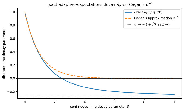
The two curves coincide for small \(\beta\) but diverge sharply for large \(\beta\): Cagan’s \(e^{-\beta}\) collapses to \(0\), whereas the exact \(\lambda_p\) turns negative and approaches \(-2 + \sqrt{3}\). For values of \(\lambda_p\) in the range estimated by Cagan (1956) and Sargent (1977), the two are close, so aggregation over time imparts at most a very small asymptotic bias to Cagan’s estimator of \(\beta\).
5. Predicting inflation using information on lagged inflation and lagged money creation#
Hansen and Sargent now turn to the bivariate moving average of the discrete-time process for inflation and money creation. A Wold moving average representation for \(((1-L)^2 p(t), (1-L)^2 m(t))' = y(t)\) is
where \(u_t\) is a \((2 \times 1)\) vector discrete-time white noise with \(Eu_t u_t' = \bar V\), where \(\bar V\) is a positive semidefinite matrix; \(u_t = y(t) - \hat E y(t)\mid y(t-1), y(t-2), \ldots\); and the eigenvalues of \(F\) are less than or equal to unity in absolute value. Given \(\Gamma_0\) and \(\Gamma_1\) from (187), \(F\) and \(\bar V\) are determined by solving
The spectral factorization theorem implies that these equations have a unique solution with the properties indicated above.
Letting \(X_t = p(t) - p(t-1)\), \(M_t = m(t) - m(t-1)\), one can write (195) as
By carrying out a series of calculations paralleling those of Muth (1960), it is straightforward to verify that (197) admits the alternative representation
From the fact that \(u\) is fundamental for \((X, M)\), it can be readily verified that there obtains the following bivariate generalization of Cagan’s adaptive expectations scheme:
The one-step-ahead prediction error vector is \(u_{t+1}\), which has covariance matrix \(\bar V\).
Representation (197) is usefully compared to the one constructed by Sargent (1977). He posited a discrete-time, bivariate, first-order moving average
where \((\varepsilon_1, \varepsilon_2)' = \varepsilon\) is a discrete-time vector white noise with arbitrary contemporaneous covariance \(E\varepsilon_t \varepsilon_t' = W\); \(\varepsilon\) is fundamental for \(((1-L) X, (1-L) M)\); and \(|\lambda| < 1\). It is evident from the first equation of (200) that Cagan’s discrete-time adaptive expectations formulation for inflation is rational, given (200). In form, (200) matches (197). A central task is now to study the relation between the \((2 \times 2)\) matrix \(F\) in (197) and the corresponding matrix
in (200). Notice that the eigenvalues of the matrix \(E\) are \(-1\) and \(-\lambda\). It can be proved that one of the eigenvalues of \(F\) in (197) is \(-1\).[3] A comparison between the value of \(-\lambda_p\) given by equation (191) and the nonunit eigenvalue of \(F\) is one interesting measure of the effects of time aggregation.
For various values of \(\beta\) and \(V = \begin{bmatrix} v_{11} & 0 \\ 0 & v_{22} \end{bmatrix}\), Hansen and Sargent calculate \(F\) and \(\bar V\), together with \(\lambda_p\) and \(\sigma_{\varepsilon p}^2\) in the univariate Wold representation for \((1-L)X\) and the analogous \(\lambda_m\) and \(\sigma_{\varepsilon m}^2\) for \((1-L) M\). Writing \(\bar v_{11}, \bar v_{22}\) for the diagonal elements of \(\bar V\) (the discrete-time one-step-ahead prediction error variances for \(X\) and \(M\) given lagged \(X\)’s and lagged \(M\)’s), the quantities
measure, respectively, the marginal assistance of lagged \(M\)’s in predicting \(X\), and of lagged \(X\)’s in predicting \(M\). These “percentage gains” are measures of the strength of the Granger causality that occurs between the discrete-time \(X\) and \(M\) processes. In the continuous-time system (182), \(m\) fails to Granger cause \(X\); however, in the discrete-time model, \(M\) will in general Granger cause \(X\) due to the effects of aggregation over time.[4]
The following code recomputes Tables 2–4 of the paper (for \(V = I\), \(V = \text{diag}(10, 1)\) and \(V = \text{diag}(1, 10)\) respectively).
def table_row(beta, v11, v22):
    G0, G1 = Gamma(beta, v11, v22)
    F, V = bivariate_factor(G0, G1)
    lam_p, s2p = ma1_factor(G0[0, 0], G1[0, 0])     # univariate (1-L)X
    lam_m, s2m = ma1_factor(G0[1, 1], G1[1, 1])     # univariate (1-L)M
    gain_p = (s2p - V[0, 0]) / s2p * 100
    gain_m = (s2m - V[1, 1]) / s2m * 100
    ev = sorted(np.linalg.eigvals(F).real, key=lambda e: abs(e + 1))
    return gain_p, gain_m, lam_p, ev[1]             # ev[0] ~ -1, ev[1] = nonunit

def print_table(v11, v22, betas):
    print(f"V = diag({v11}, {v22})")
    print(f"{'beta':>6} {'%gain p':>9} {'%gain m':>9} {'lambda_p':>10} {'eig F':>10}")
    for b in betas:
        gp, gm, lp, ef = table_row(b, v11, v22)
        print(f"{b:6.2f} {gp:9.3f} {gm:9.3f} {lp:10.6f} {ef:10.6f}")

betas = [0.05, 0.25, 0.55, 1.00, 2.00, 3.00, 5.00, 6.00, 7.00, 10.00, 20.00]
print_table(1.0, 1.0, betas)
V = diag(1.0, 1.0)
  beta   %gain p   %gain m   lambda_p      eig F
  0.05     0.000     4.753   0.951224  -0.951229
  0.25     0.000    19.658   0.778290  -0.778799
  0.55     0.003    33.177   0.572824  -0.576890
  1.00     0.032    42.150   0.351000  -0.367138
  2.00     0.396    43.473   0.071797  -0.127017
  3.00     1.216    38.863  -0.062746  -0.026334
  5.00     3.297    30.900  -0.174828   0.047553
  6.00     4.251    28.250  -0.200000   0.062746
  7.00     5.090    26.227  -0.216413   0.072361
 10.00     6.989    22.400  -0.241457   0.086582
 20.00     9.911    17.863  -0.261077   0.097335
print_table(10.0, 1.0, betas)   # Table 3
print()
print_table(1.0, 10.0, betas)   # Table 4
V = diag(10.0, 1.0)
  beta   %gain p   %gain m   lambda_p      eig F
0.05 0.000 13.559 0.951224 -0.951274
0.25 0.001 39.838 0.778290 -0.783221
0.55 0.023 47.566 0.572824 -0.608589
1.00 0.248 45.643 0.351000 -0.469338
2.00 2.120 40.205 0.071797 -0.367138
3.00 5.169 37.660 -0.062746 -0.339408
5.00 11.104 35.519 -0.174828 -0.323453
6.00 13.459 34.984 -0.200000 -0.320572
7.00 15.420 34.605 -0.216413 -0.318813
10.00 19.586 33.931 -0.241457 -0.316303
 20.00    25.502    33.161  -0.261077  -0.314473

V = diag(1.0, 10.0)
  beta   %gain p   %gain m   lambda_p      eig F
0.05 0.000 1.551 0.951224 -0.951225
0.25 0.000 7.303 0.778290 -0.778341
0.55 0.000 14.643 0.572824 -0.573236
1.00 0.003 23.201 0.351000 -0.352679
2.00 0.044 34.462 0.071797 -0.077935
3.00 0.145 38.879 -0.062746 0.052290
5.00 0.433 38.301 -0.174828 0.158938
6.00 0.575 36.157 -0.200000 0.182582
7.00 0.704 33.686 -0.216413 0.197926
10.00 1.009 26.606 -0.241457 0.221222
20.00 1.504 13.909 -0.261077 0.239363
These reproduce the published Tables 2–4 to all printed digits, with three exceptions in Table 2 (\(V = I\)) that are evidently typographical errors in the 1983 original: the nonunit eigenvalue of \(F\) at \(\beta = 1.00\) is printed as \(-0.127017\), which is a duplicate of the \(\beta = 2.00\) entry (the correct value is \(-0.367138\)); the percentage gain for \(p\) at \(\beta = 10.00\) is printed as \(6.289\) (a digit transposition of \(6.989\)); and the percentage gain for \(m\) at \(\beta = 6.00\) is printed as \(28.205\) (the recomputation gives \(28.251\)).
One outstanding characteristic that emerges is that for small values of \(\beta\), \(-\exp(-\beta)\), \(-\lambda_p\), and the nonunit eigenvalue of \(F\) are very close to each other; further, for small \(\beta\), money creation only very weakly Granger-causes inflation in the discrete-time data. On the other hand, for large values of \(\beta\), \(\exp(-\beta)\) fails to approximate \(\lambda_p\), and substantial Granger causality can extend from money creation to inflation in discrete time. The figure below plots the two percentage gains against \(\beta\) for the symmetric case \(V = I\).
bb = np.array([0.05, 0.1, 0.2, 0.35, 0.5, 0.75, 1, 1.5, 2, 3, 4, 5, 7, 10, 14, 20])
gp = np.array([table_row(b, 1.0, 1.0)[0] for b in bb])
gm = np.array([table_row(b, 1.0, 1.0)[1] for b in bb])

fig, ax = plt.subplots(figsize=(9, 5))
ax.plot(bb, gm, 'o-', lw=2, label=r'gain for $m$: lagged $X$ helps predict $M$')
ax.plot(bb, gp, 's-', lw=2, label=r'gain for $p$: lagged $M$ helps predict $X$')
ax.set_xscale('log')
ax.set_xlabel(r'continuous-time decay parameter $\beta$  (log scale)')
ax.set_ylabel('percentage gain  (Granger-causality strength)')
ax.set_title('Aggregation-over-time induced Granger causality ($V=I$)')
ax.legend()
plt.show()
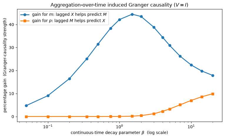
In continuous time money creation does not Granger cause inflation, yet in the point-in-time sampled discrete data it does (the “gain for \(p\)” curve is strictly positive and rises with \(\beta\)). The much larger “gain for \(m\)” reflects the strong feedback from \(p\) to \(m\) that (182) builds in to make Cagan’s mechanism optimal. For values of \(\lambda_p\) in the range estimated by Cagan and Sargent, the gain for \(p\) is small, which is comforting; for large \(\beta\), however, the effects of aggregation over time can be considerable.
6. Conclusions#
Hansen and Sargent produce a continuous-time model that solves the inverse optimal predictor problem for a continuous-time version of Cagan’s model of hyperinflation with adaptive expectations. They then deduce the restrictions this continuous-time model places on discrete-time data, obtaining exact formulas that link the parameters of the discrete-time representation to those of the continuous-time model. These formulas make it possible to evaluate the quality of the approximations that Cagan and others have used in connecting the discrete-time and continuous-time parameterizations.
The computational techniques are useful for studying the effects of aggregation over time in a variety of dynamic models under rational expectations, and in later work the authors applied them in substantially richer dynamic settings.
Appendix#
This appendix shows that the only choice of \(c_1(D)\) that has a rational Laplace transform and satisfies
is
where \(k_0\) is an arbitrary row vector constant.
The fact that no other variables Granger cause \(p\) implies that \(c_1(D)\) must take the form \(c_1(D) = c_1(D)^* k_0\) where \(c_1(D)^*\) is a scalar operator and \(k_0\) is a row vector constant that satisfies \(k_0 k_0' = 1\). Thus the fundamental representation for \(p\) can be written
where \(w(t)^* = k_0 w(t)\). The function \(c_1(s)^*\) is assumed to be rational, written as
where
Consistent with the requirement that anticipated inflation be physically realizable, the restriction \(\operatorname{Real}(\gamma_j) \leq 0\) is imposed for \(j = 1, 2, \ldots, n\). This guarantees that the vector function \(c_1^*(s)\) is analytic in the open right half plane. The assumption that \(p\) is physically realizable implies that \(m < n\).
The function \(G(s, v) = s c_1(s)^* e^{vs}\) is analytic in its first argument everywhere in the complex plane except possibly at \(\gamma_1, \gamma_2, \ldots, \gamma_n\). Let \(H_1(s, v), H_2(s, v), \ldots, H_q(s, v)\) denote the principal parts of \(G\) at the corresponding \(q\) distinct zeroes of \(\gamma(s)\). Using a result from Hansen and Sargent (1982), it follows that \([G(D, v)]_+ = H_1(D, v) + H_2(D, v) + \ldots + H_q(D, v)\).
However from (201) it is clear that \(H_j(s, v)\) cannot depend on \(v\). It follows that \(n = 2\) and \(\gamma_1 = \gamma_2 = 0\). Therefore
Computing \([D c_1(s)^* e^{vD}]_+\) gives
By equation (201),
Equation (204) implies that \(\mu_1 = -\beta\). Therefore \(c_1(D)^* = \mu_0 \dfrac{(D + \beta)}{D^2}\), which proves the desired result.
Exercises#
Exercise 23
The text states that as \(\beta \to \infty\) the exact decay parameter \(\lambda_p\) of (191) approaches \(-2 + \sqrt{3}\), while Cagan’s approximation \(e^{-\beta}\) approaches \(0\).
(a) Using (190) with \(c(0) = 2v_{11}(\tfrac{1}{3}\beta^2 + 1)\) and \(c(1) = v_{11}(\tfrac{1}{6}\beta^2 - 1)\), show analytically that \(\lim_{\beta \to \infty}\lambda_p = -2 + \sqrt{3}\). (Hint: the ratio \(c(0)/c(1) \to 4\).)
(b) Plot the absolute approximation error \(|e^{-\beta} - \lambda_p|\) as a function of \(\beta\), and confirm numerically that the error is negligible for the small-\(\beta\) range relevant to Cagan’s and Sargent’s estimates but grows toward \(|{-2+\sqrt 3}| \approx 0.27\) as \(\beta\) grows.
Solution to Exercise 23
For (a): as \(\beta \to \infty\), \(c(0)/c(1) = 2(\tfrac{1}{3}\beta^2 + 1)/(\tfrac{1}{6}\beta^2 - 1) \to 2 \cdot \tfrac{1/3}{1/6} = 4\). With \(r = c(0)/c(1) \to 4\), (190) gives \(\lambda_p = -r/2 \pm \sqrt{r^2/4 - 1} \to -2 \pm \sqrt{4 - 1} = -2 \pm \sqrt 3\). The root with \(|\lambda_p| < 1\) is \(-2 + \sqrt 3 \approx -0.267949\).
bb = np.linspace(0.01, 12, 500)
err = np.abs(np.exp(-bb) - np.array([lambda_p(b) for b in bb]))

fig, ax = plt.subplots(figsize=(9, 4.5))
ax.plot(bb, err, lw=2)
ax.axhline(abs(-2 + np.sqrt(3)), color='0.5', ls=':',
           label=r'$|{-2+\sqrt{3}}|\approx 0.268$')
ax.set_xlabel(r'$\beta$'); ax.set_ylabel(r'$|e^{-\beta} - \lambda_p|$')
ax.set_title("Error of Cagan's approximation $\\lambda \\approx e^{-\\beta}$")
ax.legend()
plt.show()

print(f"limit  -2+sqrt(3)      = {-2 + np.sqrt(3):.6f}")
print(f"lambda_p at beta=50    = {lambda_p(50.0):.6f}")
print(f"error at beta=0.5      = {abs(np.exp(-0.5) - lambda_p(0.5)):.4f}")
print(f"error at beta=10       = {abs(np.exp(-10) - lambda_p(10.0)):.4f}")
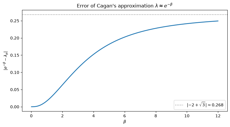
limit  -2+sqrt(3)      = -0.267949
lambda_p at beta=50    = -0.266838
error at beta=0.5      = 0.0032
error at beta=10       = 0.2415
Exercise 24
In continuous time, money creation fails to Granger cause inflation, yet aggregation over time makes money creation Granger cause inflation in the point-in-time sampled discrete data. The “percentage gain for \(p\),” \((\sigma_{\varepsilon p}^2 - \bar v_{11})/\sigma_{\varepsilon p}^2\), measures the strength of this induced causality.
(a) For the symmetric case \(V = I\), verify numerically the claim in 5. Predicting inflation using information on lagged inflation and lagged money creation that one eigenvalue of \(F\) is exactly \(-1\) for several values of \(\beta\).
(b) Compute the percentage gain for \(p\) at \(\beta = 0.35\) (a value implying \(\lambda_p\) in Cagan’s estimated range) and at \(\beta = 10\), and comment on how the strength of aggregation-induced Granger causality depends on \(\beta\).
Solution to Exercise 24
# (a) one eigenvalue of F equals -1
print("beta     eigenvalues of F")
for b in [0.35, 1.0, 5.0, 10.0]:
    G0, G1 = Gamma(b, 1.0, 1.0)
    F, V = bivariate_factor(G0, G1)
    ev = np.sort(np.linalg.eigvals(F).real)
    print(f"{b:5.2f}   {np.round(ev, 6)}")
beta     eigenvalues of F
 0.35   [-0.99995 -0.70468]
 1.00   [-0.99995  -0.367138]
 5.00   [-0.99995   0.047553]
10.00 [-0.99995 0.086582]
# (b) percentage gain for p
for b in [0.35, 10.0]:
    gp, gm, lp, ef = table_row(b, 1.0, 1.0)
    print(f"beta={b:5.2f}:  gain for p = {gp:6.3f}%   (lambda_p={lp:.4f})")
beta= 0.35: gain for p = 0.000% (lambda_p=0.7034)
beta=10.00: gain for p = 6.989% (lambda_p=-0.2415)
One eigenvalue of \(F\) sits at \(-1\) for every \(\beta\), confirming the text’s claim (it reflects the over-differencing implicit in applying \((1-L)^2\)). At \(\beta = 0.35\) the percentage gain for \(p\) is a small fraction of a percent. Money creation barely improves the inflation forecast, so Cagan’s univariate procedure loses almost nothing. At \(\beta = 10\) the gain is several percent: when the continuous-time decay is fast relative to the unit sampling interval, aggregation over time induces economically meaningful Granger causality from money creation to inflation that is entirely absent in continuous time.
References#
Cagan, P. (1956). The Monetary Dynamics of Hyperinflation, in M. Friedman, ed., Studies in the Quantity Theory of Money. Chicago: University of Chicago.
Christiano, L. (1980). Rational Expectations, Hyperinflation, and the Demand for Money. Manuscript.
Friedman, B. M. (1978). Stability and Rationality in Models of Hyperinflation. International Economic Review, 19 (February), 45–64.
Friedman, M. (1957). A Theory of the Consumption Function. Princeton: Princeton University Press.
Granger, C. W. J. (1969). Investigating Causal Relations by Econometric Models and Cross Spectral Methods. Econometrica, 37 (July), 424–438.
Hansen, L. P., and T. J. Sargent (1980). Formulating and Estimating Dynamic Linear Rational Expectations Models. Journal of Economic Dynamics and Control.
Hansen, L. P., and T. J. Sargent (1981). Linear Rational Expectations Models for Dynamically Interrelated Variables, in R. E. Lucas, Jr., and T. J. Sargent, eds., Rational Expectations and Econometric Practice. Minneapolis: University of Minnesota Press.
Hansen, L. P., and T. J. Sargent (1982). Continuous Time Models of Control, Prediction, and Rational Expectations.
Khan, M. S. (1980). Dynamic Stability in the Cagan Model of Hyperinflation. International Economic Review, 21 (October), 577–582.
Muth, J. F. (1960). Optimal Properties of Exponentially Weighted Forecasts. Journal of the American Statistical Association, 55 (June), 299–306.
Nerlove, M. (1967). Distributed Lags and Unobserved Components in Economic Time Series, in W. Fellner, et al., Ten Economic Studies in the Tradition of Irving Fisher. New York: Wiley.
Nerlove, M., D. M. Grether, and J. L. Carvalho (1979). Analysis of Economic Time Series: A Synthesis. New York: Academic Press.
Rozanov, Y. A. (1967). Stationary Random Processes. San Francisco: Holden Day.
Sargent, T. J. (1977). The Demand for Money during Hyperinflations under Rational Expectations: I. International Economic Review, 18 (February), 59–82.
Sims, C. A. (1971). Discrete Approximations to Continuous Time Distributed Lags in Econometrics. Econometrica, 39 (May), 545–564.
Sims, C. A. (1972). Money, Income and Causality. American Economic Review, 62 (September), 540–552.