22. The Dimensionality of the Aliasing Problem in Models with Rational Spectral Densities

Note

This chapter reports and paraphrases Lars Peter Hansen and Thomas J. Sargent, “The Dimensionality of the Aliasing Problem in Models with Rational Spectral Densities,” Econometrica 51 (1983), no. 2, pp. 377–387. We retell the argument in the third person, writing “Hansen and Sargent show” and “the authors,” and we preserve the original section and equation numbering. The paper contains no figures or tables. We illustrate the first-order Markov results of 4. First order Markov models numerically in Python with a worked example like the one in the companion Federal Reserve Bank of Minneapolis Staff Report No. 72.

The five theorems below are the paper’s. They are numbered in this book’s own sequence, which they continue: what the paper calls its Theorems 1 through 5 appear here as Theorem 17 through Theorem 21. Section and equation numbering remains the paper’s.

In this paper Hansen and Sargent reconsider the aliasing problem of identifying the parameters of a continuous time stochastic process from discrete time data. They analyze the extent to which restricting attention to processes with rational spectral density matrices reduces the number of observationally equivalent models, focusing on rational specifications because they are commonly employed in the analysis of time series data.

1. Introduction

It is a well known result from the theory of continuous time, covariance stationary stochastic processes that the continuous time spectral density function cannot, in general, be inferred from equispaced discrete time observations. This identification problem is commonly referred to as the aliasing phenomenon. In applications, a researcher imposes extra restrictions by adopting a finite parameterization of the spectral density function. For instance, A. W. Phillips (1959) and Hansen and Sargent (1981) used continuous time models in which the continuous time spectral density function of the observable time series is a rational function.

The purpose of the paper is to show that the specification of a rational spectral density matrix in itself goes a significantly greater distance towards resolving the aliasing problem than had previously been recognized. For some subclasses of these models, it had been thought that there is a countably infinite number of observationally equivalent models (see P. C. B. Phillips (1973)). Hansen and Sargent show that in general there is only a finite number of observationally equivalent models, and that in certain regions of the parameter space there may be no identification problem at all.

In applications, additional prior economic restrictions can be imposed on the reduced form specifications considered here. It is important to know how large a role the particular finite parameter specification of the continuous time reduced form plays, relative to the additional structural restrictions implied by economic theory, in achieving identification; the paper clarifies the roles of these two sources of identification.

Section 2 briefly describes the aliasing identification problem for a general, indeterministic, covariance stationary continuous time vector stochastic process; in this general case the class of observationally equivalent continuous time models is uncountably infinite. Section 3 takes up the more restricted case, usual in applications, of an assumed rational spectral density matrix, and indicates a machinery for proving that the class of observationally equivalent continuous time models is in general finite. Section 4 then characterizes more completely the special case studied by P. C. B. Phillips (1973), in which the true continuous time model is a first order vector Markov process; there, Hansen and Sargent show that there generally exists a discrete sampling interval fine enough for the continuous time model to be identified.

2. The aliasing problem under covariance stationarity

Consider an \(n\) dimensional continuous time stochastic process, \(x\), that is covariance stationary and linearly indeterministic. For simplicity the process is assumed to have a moving average representation

(216)\[x(t) = \int_0^\infty c(\tau)\, w(t - \tau)\, d\tau\]

where \(w\) is an \(n\) dimensional continuous time white noise process with intensity matrix \(I\) and \(c\) is an \((n \times n)\) matrix function whose elements are square integrable. The process \(w\) is assumed fundamental for \(x\), which means that linear combinations of current and past \(w\)’s span the same space as linear combinations of current and past \(x\)’s. Under these assumptions the matrix function \(c\) is unique up to post-multiplication by an orthogonal matrix.

Let \(C(s) = \int_0^\infty c(t) e^{-st}\, dt\) be the Laplace transform of \(c\). It is convenient to write representation (216) as

(217)\[x(t) = C(D)\, w(t)\]

where \(D\) is the time derivative operator. The population covariogram of \(x\) is completely summarized by the matrix function \(c\) or equivalently by its Laplace transform \(C\). Alternatively, the covariogram is characterized by its Fourier transform, the spectral density matrix. The spectral density matrix \(f\) is positive semidefinite at all frequencies \(\omega\) and is related to \(C\) by

(218)\[f(\omega) = C(i\omega) C(-i\omega)', \qquad -\infty < \omega < \infty.\]

Here the prime denotes transposition (but not conjugation). Since the \(x\) process is real, the function \(f\) satisfies

(219)\[f(\omega) = \bar f(-\omega) = \bar f(\omega)'\]

where the bar denotes conjugation.

The aliasing phenomenon for models that reside in this class can be conveniently described by using spectral density matrices. Let \(F\) denote the spectral density matrix of the process \(X\) obtained by observing \(x\) at integer points in time. It is known that \(f\) and \(F\) are linked by the following formula:

(220)\[F(\omega) = \sum_{j=-\infty}^{+\infty} f(\omega + 2\pi j).\]

Since \(F\) completely summarizes the population covariance properties of \(X\), formula (220) implies that the function \(f\) cannot be inferred from the discrete time data. This can be seen by noting that alternative Hermitian, positive semidefinite matrix functions \(f^*\) can be constructed that satisfy

(221)\[F(\omega) = \sum_{j=-\infty}^{+\infty} f^*(\omega + 2\pi j), \qquad f^*(\omega) = \bar f^*(-\omega),\]

and hence are observationally equivalent to \(f\). Corresponding to each function \(f^*\) is a matrix of square integrable functions \(c^*\) with Laplace transforms \(C^*\) such that \(f^*(\omega) = C^*(i\omega) C^*(-i\omega)'\), and such that if \(w^*\) is an \(n\) dimensional continuous time white noise process with intensity matrix \(I\), then \(w^*\) is fundamental for \(x^*\) where \(x^*(t) = C^*(D) w^*(t)\). Although the matrix function \(c^*\) cannot be obtained from \(c\) by post multiplying \(c\) by an orthogonal matrix, \(c^*\) is observationally equivalent to \(c\) with discrete time data. This is the conventional formulation of the aliasing problem in time series analysis.

The models in (216) are in general infinite parameter models, with the parameters in \(c\) being the objects whose identification is sought. At this level of generality, the aliasing problem is a local identification problem, in the sense that there are observationally equivalent parameters \(c^*\) satisfying (220) and (221) that are arbitrarily close to the true parameter \(c\). The relevant measure of distance is the matrix \(L_2\) norm

\[ \int_0^\infty \operatorname{trace}\{[c(\tau) - c^*(\tau)][c(\tau) - c^*(\tau)]'\}\, d\tau. \]

There is an overwhelming number of \(c^*\)’s that are observationally equivalent to \(c\). In fact, this number is uncountable.[1] Thus, at the general level of the model (216), the dimensionality of the class of observationally equivalent models given equispaced discrete time observations is uncountable.

Illustration: spectral folding and observational equivalence

The folding formula (220) is the engine of the aliasing problem. We illustrate it with a scalar first order Markov process \(Dx(t) = -a\, x(t) + \epsilon(t)\) (intensity \(v\)), whose continuous time spectral density is the Lorentzian \(f(\omega) = v/(a^2 + \omega^2)\), the same Ornstein–Uhlenbeck spectrum met in 8. Spectral Densities and 17. Discrete Sampling: The Folding Formula. Sampling at the integers folds all of the \(2\pi\)-shifted copies \(f(\omega + 2\pi j)\) down onto the band \([-\pi, \pi]\). As a check, the resulting \(F(\omega)\) must equal the spectral density of the implied discrete time first order autoregression \(X_t = e^{-a} X_{t-1} + \eta_t\), namely \(F(\omega) = \sigma_\eta^2 / |1 - e^{-a} e^{-i\omega}|^2\) with \(\sigma_\eta^2 = v(1 - e^{-2a})/(2a)\).

import numpy as np
import matplotlib.pyplot as plt

a, v = 1.5, 1.0
f_cont = lambda w: v / (a**2 + w**2)                       # continuous OU spectrum

def F_fold(w, N=2000):                                     # folding formula (5)
    j = np.arange(-N, N + 1)[:, None]
    return f_cont(np.atleast_1d(w)[None, :] + 2*np.pi*j).sum(axis=0)

sig2 = v * (1 - np.exp(-2*a)) / (2*a)                      # discrete AR(1) innovation var
F_exact = lambda w: sig2 / (1 - 2*np.exp(-a)*np.cos(w) + np.exp(-2*a))

w_wide = np.linspace(-5*np.pi, 5*np.pi, 1600)
w_band = np.linspace(-np.pi, np.pi, 400)

fig, (ax1, ax2) = plt.subplots(2, 1, figsize=(9, 7))
ax1.axvspan(-np.pi, np.pi, color='C2', alpha=0.10, label=r'observable band $[-\pi,\pi]$')
for j in range(-2, 3):
    ax1.plot(w_wide, f_cont(w_wide + 2*np.pi*j), color='0.6', lw=1,
             ls='-' if j == 0 else '--')
ax1.plot(w_wide, f_cont(w_wide), 'C0', lw=2.2, label=r'$f(\omega)=v/(a^2+\omega^2)$')
for k in range(-5, 6, 2):
    ax1.axvline(k*np.pi, color='0.85', lw=0.6)
ax1.set_xlabel(r'$\omega$'); ax1.set_ylabel('continuous density + copies')
ax1.set_title(r'Continuous spectral density and its $2\pi$-shifted copies $f(\omega+2\pi j)$')
ax1.legend(loc='upper right', fontsize=9)

ax2.plot(w_band, F_fold(w_band), 'C0', lw=2.2,
         label=r'$F(\omega)=\sum_j f(\omega+2\pi j)$  (eq. 5)')
ax2.plot(w_band[::20], F_exact(w_band[::20]), 'ro', ms=5,
         label='exact discrete AR(1) spectrum')
ax2.set_xlabel(r'$\omega$'); ax2.set_ylabel(r'$F(\omega)$')
ax2.set_title('Discrete (integer-sampled) spectrum: the aliased fold of $f$')
ax2.legend(fontsize=9)
plt.tight_layout(); plt.show()

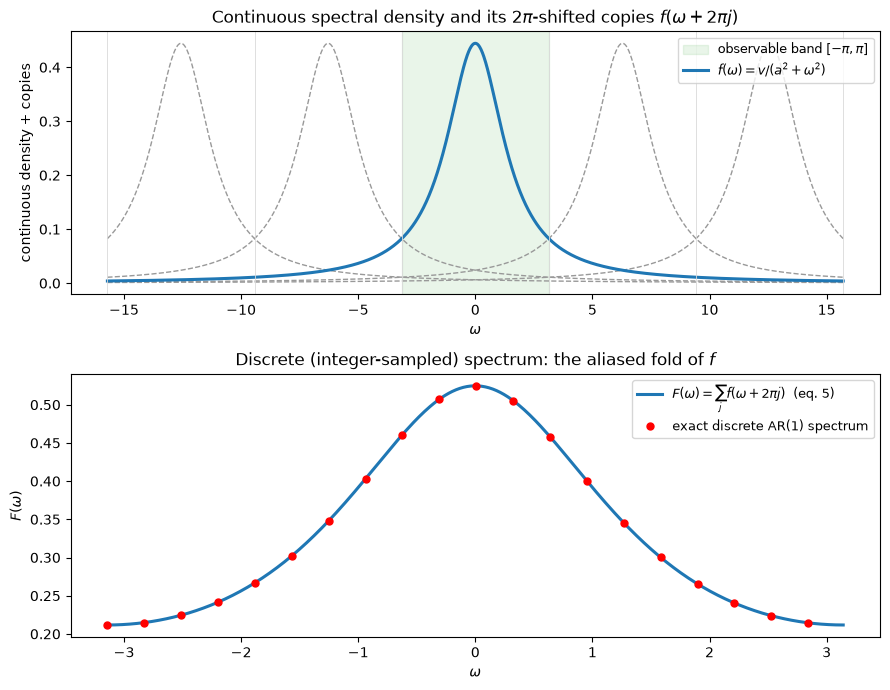
The folded sum reproduces the discrete AR(1) spectrum exactly, confirming (220). Now we exhibit the non-identification directly: a different continuous spectral density \(f^*\) that folds to the same \(F\). Following the bandlimited construction of [1] (with \(\omega^* = \pi\)), put all of \(f^*\)’s power in the high-frequency band \(\pi < |\omega| < 3\pi\), setting it equal to \(\tfrac{1}{2} F\) there. Its fold onto \([-\pi, \pi]\) then equals \(F\), so \(x\) and \(x^*\) are observationally indistinguishable from integer-sampled data even though their continuous time spectra differ completely. One is a smooth low-frequency Lorentzian; the other is concentrated entirely at high frequencies.

The device that manufactures \(x^*\) is the band-pass window \(B_{cd}(w)\) of 10. The Cramér Representation, applied at frequencies above the Nyquist rate. There it was used to decompose a process into orthogonal frequency bands, each carrying its own share of the variance; here it is used in reverse, to assemble a process whose entire variance sits in bands that sampling folds down on top of the observable one. The two processes have the same total power, and the variance printed below is \(v/2a\) for both. Folding preserves the sum of the band variances and destroys only the information about how the sum was divided among them.

def f_star(w):
    w = np.atleast_1d(w).astype(float); out = np.zeros_like(w)
    band = (np.abs(w) > np.pi) & (np.abs(w) < 3*np.pi)
    out[band] = 0.5 * F_exact(w[band])        # F_exact is 2*pi-periodic
    return out

w_in = np.linspace(-np.pi + 1e-3, np.pi - 1e-3, 400)
F_fold_star = lambda w: sum(f_star(w + 2*np.pi*j) for j in range(-2, 3))

print("max |fold(f*) - F| on (-pi, pi):", np.max(np.abs(F_fold_star(w_in) - F_exact(w_in))))
wg = np.linspace(-3*np.pi, 3*np.pi, 600001)
print(f"continuous variance of f   = {v/(2*a):.5f}")
print(f"continuous variance of f*  = {np.trapz(f_star(wg), wg)/(2*np.pi):.5f}")

fig, (ax1, ax2) = plt.subplots(2, 1, figsize=(9, 7))
ax1.axvspan(-np.pi, np.pi, color='C2', alpha=0.10)
ax1.plot(w_wide, f_cont(w_wide), 'C0', lw=2.2, label=r'$f$  (Ornstein–Uhlenbeck)')
ax1.plot(w_wide, f_star(w_wide), 'C3', lw=2.2,
         label=r'$f^*$  (bandlimited, $\pi<|\omega|<3\pi$)')
ax1.set_xlabel(r'$\omega$'); ax1.set_ylabel('continuous density')
ax1.set_title('Two very different continuous spectral densities')
ax1.legend(fontsize=9)

ax2.plot(w_in, F_fold_star(w_in), 'C3', lw=5, alpha=0.45, label=r'fold of $f^*$')
ax2.plot(w_in, F_fold(w_in), 'C0', lw=2, label=r'fold of $f$')
ax2.set_xlabel(r'$\omega$'); ax2.set_ylabel(r'$F(\omega)$')
ax2.set_title('…with identical discrete spectrum: observationally equivalent')
ax2.legend(fontsize=9)
plt.tight_layout(); plt.show()

max |fold(f*) - F| on (-pi, pi): 2.220446049250313e-16
continuous variance of f   = 0.33333

---------------------------------------------------------------------------
AttributeError                            Traceback (most recent call last)
Cell In[2], line 13
      9 
     10 print("max |fold(f*) - F| on (-pi, pi):", np.max(np.abs(F_fold_star(w_in) - F_exact(w_in))))
     11 wg = np.linspace(-3*np.pi, 3*np.pi, 600001)
     12 print(f"continuous variance of f   = {v/(2*a):.5f}")
---> 13 print(f"continuous variance of f*  = {np.trapz(f_star(wg), wg)/(2*np.pi):.5f}")
     14 
     15 fig, (ax1, ax2) = plt.subplots(2, 1, figsize=(9, 7))
     16 ax1.axvspan(-np.pi, np.pi, color='C2', alpha=0.10)

File /opt/hostedtoolcache/Python/3.11.16/x64/lib/python3.11/site-packages/numpy/__init__.py:792, in __getattr__(attr)
    789     import numpy.char as char
    790     return char.chararray
--> 792 raise AttributeError(f"module {__name__!r} has no attribute {attr!r}")

AttributeError: module 'numpy' has no attribute 'trapz'

The two continuous processes have the same total power (variance \(v/2a\)) and the same integer-sampled spectrum, yet different continuous spectra; varying \(\omega^*\) over the uncountable set \(\{\omega^* > \pi\}\) generates uncountably many such aliases. This is the uncountable dimensionality of the general covariance-stationary case. The rest of the paper shows how far the rational and Markov restrictions shrink this class, from uncountable to finite, and often to a single point.

3. The aliasing problem with a rational spectral density matrix

In applications it is necessary to adopt a finite parameterization of the matrix function \(c\). A convenient parameterization is to assume that \(c\) has a rational Laplace transform, giving the rational spectral densities of 8. Spectral Densities and the sum-of-exponentials kernels of the linear stochastic differential equations of 11. Linear Stochastic Differential Equations. In particular, suppose that

(222)\[C(s) = \frac{(G_0 + G_1 s + \cdots + G_{q-1} s^{q-1})}{(s - \lambda_1)(s - \lambda_2) \cdots (s - \lambda_q)} = \frac{G(s)}{g(s)}\]

where \(G_0, G_1, \ldots, G_{q-1}\) are \((n \times n)\) matrices, \(\lambda_1, \lambda_2, \ldots, \lambda_q\) are distinct complex numbers with nonzero real parts, and \(g(s)\) is the lowest common denominator polynomial for the elements of \(C(s)\). The zeroes of \(\det G(s)\) are assumed to have negative real parts, and for each \(j\), \(\lambda_j = \bar\lambda_{k}\) for some index \(k\). Finally, any two \(\lambda\)’s with the same real part are assumed not to have imaginary parts that differ by an integer multiple of \(2\pi i\). The \(\lambda\)’s are called the poles of the complex matrix function \(C\).

Hansen and Sargent examine the spectral density matrix of a process with a \(C\) that satisfies specification (222). Following an approach used by A. W. Phillips (1959), they form the partial fractions representation of the matrix function \(h\),

(223)\[h(s) = C(s) C(-s)' = \sum_{j=1}^q \left[ \frac{Q_j}{s - \lambda_j} + \frac{Q_j'}{-s - \lambda_j} \right]\]

where

\[ Q_j = \frac{G(\lambda_j) G(-\lambda_j)'}{g_j\, g_{-j}\, (-2\lambda_j)}, \qquad g_j = \lim_{s \to \lambda_j} \frac{g(s)}{(s - \lambda_j)}, \qquad g_{-j} = \lim_{s \to \lambda_j} \frac{g(-s)}{(-s - \lambda_j)}. \]

Note that if \(\lambda_k\) is the complex conjugate of \(\lambda_j\), then the elements of \(Q_k\) are complex conjugates of the elements of \(Q_j\). The spectral density matrix of \(x\) is \(f(\omega) = h(i\omega)\), and the autocovariance function, which equals the inverse Fourier transform of \(f\), is

(224)\[\begin{split}r(\tau) = \begin{cases} \displaystyle\sum_{j=1}^q Q_j\, e^{\lambda_j \tau} & \text{for } \tau \geq 0, \\[1ex] r(-\tau)' & \text{for } \tau < 0. \end{cases}\end{split}\]

Suppose one wishes to construct a function \(r^*\) that is distinct from \(r\) but can be written in the form (224) and is equal to \(r\) at integer values of \(\tau\). Such an \(r^*\) is a candidate for a continuous time autocovariance function that is observationally equivalent to \(r\). To generate a family of such \(r^*\)’s, the authors use equation (224) and the fact that \(e^{2\pi i \tau} = 1\) for any integer \(\tau\). Since the function \(r\) at integer values of \(\tau\) can be inferred from discrete time data, it is evident that the complex matrices \(Q_j\) and the complex numbers \(\rho_j\) are identifiable from discrete time data where \(\rho_j = e^{\lambda_j}\). It follows that the real parts of the poles \(\lambda_j\) are just the real logarithms of \(|\rho_j|\). Hence the real parts of the poles are identifiable from discrete time data. On the other hand, the imaginary parts of the poles are not necessarily identifiable. If at least one of the poles is complex, then one can construct a countable infinity of real matrix functions \(r^*\) of the form given in (224) that are equal to \(r\) at integer values of \(\tau\). Thus, suppose that the first two \(\lambda\)’s form a complex conjugate pair. Let \(\lambda_1^k = \lambda_1 + 2\pi i k\) and \(\lambda_2^k = \lambda_2 - 2\pi i k\). Now form the functions

\[\begin{split} r_k(\tau) = \begin{cases} Q_1 e^{\lambda_1^k \tau} + Q_2 e^{\lambda_2^k \tau} + \displaystyle\sum_{j=3}^q Q_j e^{\lambda_j \tau} & \text{for } \tau \geq 0, \\[1ex] r_k(-\tau)' & \text{for } \tau < 0. \end{cases} \end{split}\]

The matrix functions \(r_k\) equal \(r\) at integer values of \(\tau\), so Hansen and Sargent have generated a countable sequence of candidate autocovariance functions for observationally equivalent models. However, for these functions to be legitimate autocovariance functions of a continuous time process, it is necessary and sufficient that their continuous Fourier transforms be positive semidefinite at all frequencies. That is,

\[\begin{split} \begin{aligned} f_k(\omega) &= \frac{Q_1}{i\omega - \lambda_1^k} + \frac{Q_1'}{-i\omega - \lambda_1^k} + \frac{Q_2}{i\omega - \lambda_2^k} + \frac{Q_2'}{-i\omega - \lambda_2^k} \\ &\quad + \sum_{j=3}^q \left[ \frac{Q_j}{i\omega - \lambda_j} + \frac{Q_j'}{-i\omega - \lambda_j} \right] \end{aligned} \end{split}\]

must be positive semidefinite for all values of \(\omega\). While this condition is met for \(f\), it will not in general be satisfied for \(f_k\). In fact, except in singular cases, only a finite number of observationally equivalent models can be generated in this fashion, as the following theorem states.

Theorem 17

If \((Q_1 + Q_1')\) is not positive semidefinite, then there is a positive integer \(k^*\) such that when \(|k| \geq k^*\), \(f_k\) is not a spectral density matrix for a continuous time process.

The condition that \((Q_1 + Q_1')\) be positive semidefinite will be met only for singular examples of the \(C(s)\) as given by (222). Theorem 17 indicates the difficulty in generating a countable sequence of observationally equivalent continuous time models without violating the requirement that the implied continuous time spectral density matrix be positive semidefinite at all frequencies. When \(C\) has only one complex conjugate pair of poles, this theorem implies that in general there will only be a finite number of observationally equivalent models. The strategy described above for constructing observationally equivalent continuous time models does not exhaust all possible ways of constructing such models when there is more than one complex conjugate pair of poles. Instead, the authors present a comprehensive analysis of the dimensionality of the special case of (222) studied by P. C. B. Phillips, which is taken up in the following section.

4. First order Markov models

Hansen and Sargent now study identification of the parameters of continuous time first order Markov processes from discrete time data, building upon and modifying P. C. B. Phillips’s (1973) characterization of the aliasing phenomenon for this class of models.

Consider an \(x\) process that can be represented

(225)\[Dx(t) = A_0\, x(t) + \epsilon(t),\]

where \(\epsilon\) is a continuous time vector white noise with intensity matrix \(V_0\). The square matrix \(A_0\) is real and has eigenvalues whose real parts are negative. From (225) one can derive a fundamental moving average representation as follows. Assume \(V_0\) has full rank and factor it as \(V_0 = U_0' U_0\). Solving (225) for \(x(t)\) gives

(226)\[x(t) = \frac{\operatorname{adj}[DI - A_0]\, U_0'}{\det[DI - A_0]}\, w(t),\]

where \(w(t) = U_0'^{-1} \epsilon(t)\) and adj denotes adjoint. Rewrite (226) as \(x(t) = C(D) w(t)\) where \(C(D) = \dfrac{\operatorname{adj}[DI - A_0]}{\det[DI - A_0]} U_0'\). The white noise vector \(w(t)\) has intensity matrix \(I\), the poles of \(C(s)\) are just the eigenvalues of \(A_0\), and the \(Q_j\) matrices in the matrix partial fractions decomposition of \(h(s) = C(s) C(-s)'\) are rank one matrices formed from the eigenvectors of \(A_0\). Rather than discuss identification with the machinery of Section 3, Hansen and Sargent adopt an alternative more convenient for these first order Markov models, one used by Phillips (1973).

The discrete time process obtained by sampling \(x\) at the integers has a first order autoregressive representation

(227)\[X(t) = B_0\, X(t-1) + \eta(t)\]

where

(228)\[B_0 = \exp A_0, \qquad \eta(t) = \int_0^1 \exp(A_0 \tau)\, \epsilon(t - \tau)\, d\tau.\]

By the white noise nature of \(\epsilon\), it follows that \(\eta\) is a discrete time vector white noise disturbance when sampled at the integers. This \(\eta\) is the discrete-time innovation of 15. State-Space Models, the Kalman Filter, and Spectral Factorization for the special case in which the state is observed without measurement error, so that the filter is exact and the innovation is simply the accumulated process noise over one sampling interval. The contemporaneous covariance matrix of \(\eta(t)\) is

(229)\[W_0 = \int_0^1 \exp(A_0 \tau)\, V_0\, \exp(A_0' \tau)\, d\tau.\]

As noted by Phillips (1973), the covariance properties of \(x\) sampled at the integers are completely characterized by \((B_0, W_0)\). Given the pair \((B_0, W_0)\), which is estimable from discrete time data,[2] the goal is to identify the covariance properties of the continuous time process, which are completely characterized by \((A_0, V_0)\). The version of the aliasing phenomenon considered by Phillips (1973) is simply that, given \((B_0, W_0)\), one cannot in general solve uniquely for \((A_0, V_0)\) using equations (228) and (229). Hansen and Sargent seek to characterize the dimensionality of the class of \((A_0, V_0)\) pairs consistent with a given \((B_0, W_0)\).

To begin, consider equation (228) and ask whether the matrix equation

(230)\[\exp A^* = B_0 = \exp A_0\]

implies that \(A^* = A_0\). Without restrictions on the matrix \(A^*\), the answer is in general no. If the matrix \(A_0\) has complex eigenvalues, then there is a countable infinity of matrices \(A^*\) that satisfy (230). To see this, assume that the eigenvalues of \(A_0\) are distinct and write the spectral decomposition of \(A_0\),

(231)\[A_0 = T \Lambda T^{-1},\]

where \(\Lambda\) is a diagonal matrix of eigenvalues of \(A_0\) and \(T\) is a matrix of eigenvectors of \(A_0\). Without loss of generality, the first \(n - 2m\) diagonal elements may be taken real, with the remainder occurring in complex conjugate pairs as \(\lambda_{n-2m+1}, \ldots, \lambda_{n-m}, \lambda_{n-2m+1} = \bar\lambda_{n-m+1}, \ldots, \lambda_n = \bar\lambda_{n-m}\). The eigenvalues of \(A_0\) are assumed not to differ by integer multiples of \(2\pi i\). Following Phillips (1973) and Coddington and Levinson (1955), if a matrix \(A^*\) satisfies (230), then

(232)\[\begin{split}A^* = A_0 + 2\pi i\, T \begin{bmatrix} 0 & 0 & 0 \\ 0 & P & 0 \\ 0 & 0 & -P \end{bmatrix} T^{-1}\end{split}\]

where \(P\) is an \((m \times m)\) diagonal matrix of integers. Any choice of integers for the diagonal elements of \(P\) will give rise to a solution of the matrix equation (230).

Phillips (1973) asserted that the pair \((A_0, V_0)\) is identifiable in \((B_0, W_0)\) if and only if the matrix \(A_0\) is identifiable in \(B_0\). This assertion would be true if, given a real valued matrix \(A^*\) of the form specified in (232), it were possible to find a positive semidefinite matrix \(V^*\) such that

(233)\[\int_0^1 \exp(A^* \tau)\, V^*\, \exp(A^{*\prime} \tau)\, d\tau = \int_0^1 \exp(A_0 \tau)\, V_0\, \exp(A_0' \tau)\, d\tau.\]

Now Phillips’s equation 4 shows how to compute a \(V^*\) satisfying (233) as a function of \(A^*\) and \(W_0\). However, there is no guarantee that the resulting \(V^*\) is positive semidefinite, and so it need not be a legitimate intensity matrix of a white noise process. This fact indicates the presence of extra identifying information about \(A_0\) in the discrete innovation covariance matrix \(W_0\), information summarized in equation (229).[3] It follows that Phillips’s characterization of the identification problem must be modified to take account of the information about \(A_0\) that is contained in \(W_0\). The question of whether \(V^*\) is positive semidefinite is equivalent to the question of whether the implied continuous time spectral density matrix is positive semidefinite at all frequencies.

Phillips asserted that if \(A_0\) has complex eigenvalues, then without additional restrictions, there is a countable infinity of pairs \(\{(A_k, V_k)\}_{k=1}^\infty\) that are observationally equivalent to \((A_0, V_0)\) given discrete time data. Actually, however, the number of pairs \((A_k, V_k)\) that are observationally equivalent to \((A_0, V_0)\) is, except for singular cases, at most finite, and in some cases equal to one even if \(A_0\) has complex eigenvalues. Hansen and Sargent substantiate this claim with four theorems.

Theorem 18

If there exists an \(A^* \neq A_0\) such that (i) \(\exp A^* = B_0\), (ii) \(\int_0^1 \exp(A^* \tau) V_0 \exp(A^{*\prime} \tau)\, d\tau = W_0\), then there is an infinite sequence of distinct matrices \(\{A_k\}_{k=1}^\infty\) that satisfy (i) and (ii).

Theorem 18 states that if one can find an \(A^*\) of the form given in (232) that also satisfies (233) for \(V^* = V_0\), then there is a countable infinity of observationally equivalent pairs \(\{(A_k, V_k)\}_{k=1}^\infty\) with \(V_k = V_0\). That is, each of the \(A_k\) matrices is associated with the same intensity matrix \(V_0\). The key feature is that the intensity matrix remains unaltered as one entertains admissible alterations of the continuous time coefficient matrix.

Theorem 18 delineates one class of circumstances in which there is a countably infinite number of continuous time models that are consistent with the discrete time observations. It happens that the class identified in Theorem 18 contains the only cases in which an infinite number of continuous time models are consistent with the discrete time observations. This is established in Theorem 19.

Theorem 19

If there does not exist an \(A^* \neq A_0\) such that (i) and (ii) of Theorem 18 are satisfied, then there is only a finite number of distinct pairs \((A_k, V_k)\) that satisfy (i’) \(\exp A_k = B_0\), (ii’) \(\int_0^1 \exp(A_k \tau) V_k \exp(A_k' \tau)\, d\tau = W_0\), (iii’) \(V_k\) is positive semidefinite.

The important feature of Theorem 19 is requirement (iii’). Phillips has shown that if \(A_0\) has complex eigenvalues, then there is a countable infinity of \(\{(A_k, V_k)\}\) that satisfy (i’) and (ii’). Theorem 19 indicates that when \(V_k\) is required to be positive semidefinite, then in many circumstances there is only a finite number of pairs \((A_k, V_k)\) that also satisfy (i’) and (ii’).

It remains to determine the size of the class of cases for which there is a countable infinity of observationally equivalent continuous time models. This question is answered by Theorem 20.

Theorem 20

If \(R_0 = T^{-1} V_0\, \bar T'^{-1}\) does not have any zero elements, then there is at most a finite number of distinct pairs \((A_k, V_k)\) that satisfy (i’), (ii’), and (iii’) of Theorem 19.

Theorem 20 indicates that the class of cases in which there is a countable infinity of \((A_k, V_k)\) that are observationally equivalent to \((A_0, V_0)\) is singular. Only when \(R_0\) has zero elements can this occur. Furthermore, there are many situations in which \(R_0\) has zero elements and there is still only a finite number of observationally equivalent models.

Hansen and Sargent now investigate the limiting behavior as the continuous time process is sampled more frequently. Let \(h\) denote the length of time between observations, with \(X(t) = x(ht)\) for integer values of \(t\). In this circumstance

\[ B_0 = \exp(h A_0), \qquad W_0 = \int_0^h \exp(A_0 \tau)\, V_0\, \exp(A_0' \tau)\, d\tau. \]

The question is what happens to the number of observationally equivalent models as \(h\) gets small. Theorem 21 provides an answer to this question.

Theorem 21

If \(R_0 = T^{-1} V_0\, \bar T'^{-1}\) does not have any zero elements, then there is an \(h^*\) such that for \(h \leq h^*\) the model \((A_0, V_0)\) is identified from \((B_0, W_0)\).

The content of Theorem 21 is that except for singular cases, it is possible to sample the continuous time process at fine enough time intervals so that the aliasing problem vanishes. This result is in sharp contrast to what happens to identification in cases in which the underlying continuous time process is a priori restricted only to be covariance stationary. In the latter circumstance, there is an uncountable infinity of observationally equivalent models for any choice of \(h\).

To summarize, Hansen and Sargent show that even when \(A_0\) has complex eigenvalues, equations (230) and (233) will in most circumstances have only a finite number of solutions, and in many cases only one. The upshot is that for many values of the continuous time parameters \((A_0, V_0)\) the identification problem is less extensive than Phillips’s characterization suggested.

A numerical illustration

We illustrate Theorem 18 through Theorem 21 with a concrete two-dimensional example. Let the continuous time generator be a damped rotation,

\[\begin{split} A_0 = \begin{bmatrix} -a & \omega \\ -\omega & -a \end{bmatrix}, \end{split}\]

which has the complex conjugate eigenvalues \(-a \pm i\omega\), and let \(V_0\) be a (full rank) intensity matrix. Sampling at interval \(h\), the discrete time data are summarized by \(B_0 = \exp(hA_0)\) and the innovation covariance \(W_0 = \int_0^h \exp(A_0\tau) V_0 \exp(A_0'\tau)\, d\tau\).

Because \(\cos\) and \(\sin\) are \(2\pi\)-periodic, every aliased generator

\[\begin{split} A_k = \begin{bmatrix} -a & \omega + 2\pi k/h \\ -(\omega + 2\pi k/h) & -a \end{bmatrix}, \qquad k \in \mathbb{Z}, \end{split}\]

satisfies \(\exp(h A_k) = B_0\): at the level of the discrete autoregressive matrix alone there is a countable infinity of observationally equivalent continuous time coefficient matrices (Phillips’s result). The Hansen–Sargent refinement is that each candidate \(A_k\) must also reproduce the discrete innovation covariance \(W_0\) through a positive semidefinite intensity matrix \(V_k\) solving (233). As we now compute, only finitely many \(k\) pass this test.

import numpy as np
import matplotlib.pyplot as plt
from scipy.linalg import expm

def A_mat(a, omega):
    """Damped-rotation generator with eigenvalues -a ± i*omega."""
    return np.array([[-a, omega], [-omega, -a]])

def integral_map(A, h):
    """Linear map M with vec(W) = M vec(V) for  W = ∫_0^h e^{Aτ} V e^{A'τ} dτ
    (column-stacking vec), via the Kronecker-sum closed form
        ∫_0^h e^{Aτ}⊗e^{Aτ} dτ = (A⊕A)^{-1}[e^{Ah}⊗e^{Ah} − I]."""
    n = A.shape[0]; I = np.eye(n)
    K = np.kron(A, I) + np.kron(I, A)
    return np.linalg.solve(K, np.kron(expm(A*h), expm(A*h)) - np.eye(n*n))

def W_from_V(A, V, h):
    return (integral_map(A, h) @ V.flatten('F')).reshape(A.shape, order='F')

def V_from_W(A, W, h):
    return np.linalg.solve(integral_map(A, h), W.flatten('F')).reshape(A.shape, order='F')

# True continuous-time model: fast rotation (omega) relative to damping (a)
a, omega = 0.2, 6.0
V0 = np.array([[1.0, 0.3], [0.3, 0.8]])
h = 1.0                                  # sample at the integers

A0 = A_mat(a, omega)
B0 = expm(h * A0)
W0 = W_from_V(A0, V0, h)

print("B0 = exp(h A0):\n", np.round(B0, 5))
print("W0 (discrete innovation covariance):\n", np.round(W0, 5))

print(f"\n{'k':>3} | exp(h A_k)=B0? | smallest eig of V_k | admissible (V_k PSD)?")
admissible = []
for k in range(-6, 7):
    Ak = A_mat(a, omega + 2*np.pi*k/h)
    same = np.allclose(expm(h*Ak), B0, atol=1e-8)
    Vk = V_from_W(Ak, W0, h); Vk = (Vk + Vk.T)/2
    mineig = np.linalg.eigvalsh(Vk).min()
    ok = mineig > -1e-9
    if ok: admissible.append(k)
    print(f"{k:3d} | {str(same):5s}          | {mineig: .5f}           | {ok}")

print(f"\nObservationally equivalent continuous-time models at h={h}: "
      f"{len(admissible)}  (k = {admissible})")

Every \(A_k\) reproduces the discrete autoregressive matrix \(B_0\) exactly, yet only the five values \(k \in \{-3, -2, -1, 0, 1\}\) deliver a positive semidefinite intensity \(V_k\). The class of observationally equivalent continuous time models is therefore finite: five, not the countable infinity that the autoregressive matrix alone would suggest, exactly as Theorem 19 and Theorem 20 assert. The figure plots the smallest eigenvalue of \(V_k\) against \(k\); admissibility is the shaded region where it is nonnegative.

ks = np.arange(-8, 9)
mineigs = []
for k in ks:
    Ak = A_mat(a, omega + 2*np.pi*k/h)
    Vk = V_from_W(Ak, W0, h); Vk = (Vk + Vk.T)/2
    mineigs.append(np.linalg.eigvalsh(Vk).min())
mineigs = np.array(mineigs)

fig, ax = plt.subplots(figsize=(9, 5))
ax.axhspan(0, max(mineigs)*1.1, color='C2', alpha=0.10, label='admissible ($V_k$ PSD)')
ax.axhline(0, color='k', lw=0.8)
ax.plot(ks, mineigs, 'o-', lw=1.5)
ax.plot(0, mineigs[ks == 0], 'D', ms=10, color='C3', label='true model ($k=0$)')
ax.set_xlabel('alias index $k$')
ax.set_ylabel(r'smallest eigenvalue of implied intensity $V_k$')
ax.set_title('Aliased continuous-time models: only finitely many have a legitimate intensity')
ax.legend()
plt.show()

Now we vary the sampling interval \(h\). Sampling faster shrinks the spacing \(2\pi/h\) between aliased rotation rates, but it also makes the off-diagonal compensation demanded of \(V_k\) ever more severe; the number of admissible models falls and eventually reaches one. This is Theorem 21: fast enough sampling identifies the continuous time model.

def n_admissible(a, omega, V0, h, K=60):
    A0 = A_mat(a, omega); W0 = W_from_V(A0, V0, h)
    n = 0
    for k in range(-K, K+1):
        Ak = A_mat(a, omega + 2*np.pi*k/h)
        Vk = V_from_W(Ak, W0, h); Vk = (Vk + Vk.T)/2
        if np.linalg.eigvalsh(Vk).min() > -1e-9:
            n += 1
    return n

hs = np.linspace(0.05, 4.0, 80)
counts = [n_admissible(a, omega, V0, h) for h in hs]

fig, ax = plt.subplots(figsize=(9, 5))
ax.plot(hs, counts, lw=2)
ax.axhline(1, color='0.5', ls=':', label='identified (one model)')
ax.set_xlabel('sampling interval $h$')
ax.set_ylabel('number of observationally equivalent models')
ax.set_title('{prf:ref}`thm-hs-5`: faster sampling resolves the aliasing problem')
ax.legend()
plt.show()

h_star = max(h for h, c in zip(hs, counts) if c == 1)
print(f"For this example the model is identified once h <= {h_star:.3f} "
      f"(only the true continuous-time model survives).")

The count of observationally equivalent models is always finite, never the uncountable infinity of the purely covariance-stationary case of §2, and it collapses to one as \(h \to 0\).

5. Conclusion

The preceding results provide a notion of the role of the prior assumption of a rational spectral density matrix, or a vector first order Markov process, in resolving the aliasing identification problem. Previously, it was known that in the general covariance stationary case the dimensionality of the identification problem was uncountably infinite; and it was believed that for the rational spectral density case, in particular the first-order Markov case, the dimensionality was countably infinite. Realizing that in this latter case the dimensionality is finite better indicates the relative contributions of the restriction to a rational spectral density matrix, on the one hand, and any additional prior economic restrictions such as exclusion or cross-equation restrictions, on the other hand, in achieving identification. The role of additional prior restrictions of various kinds in achieving unique identification is described in Phillips (1973) and Hansen and Sargent (1981).

Exercises

Exercise 28

The discrete autoregressive matrix \(B_0 = \exp(A_0)\) on its own leaves a countable infinity of continuous time coefficient matrices undetermined; adding the discrete innovation covariance \(W_0\), and insisting that the implied intensity be positive semidefinite, cuts this down to a finite set. Make this contrast quantitative for the example of 4. First order Markov models (\(a = 0.2\), \(\omega = 6\), \(V_0 = \begin{bmatrix} 1 & 0.3 \\ 0.3 & 0.8 \end{bmatrix}\), \(h = 1\)):

(a) Confirm that \(\exp(A_k) = B_0\) for \(k = -10, \ldots, 10\) (so the autoregressive matrix alone admits infinitely many continuous time models).

(b) Count how many of those \(A_k\) are accompanied by a positive semidefinite \(V_k\). Verify that the true model \(k = 0\) is among them.

Solution to Exercise 28

a, omega, h = 0.2, 6.0, 1.0
V0 = np.array([[1.0, 0.3], [0.3, 0.8]])
A0 = A_mat(a, omega); B0 = expm(h*A0); W0 = W_from_V(A0, V0, h)

all_match = all(np.allclose(expm(h*A_mat(a, omega + 2*np.pi*k/h)), B0, atol=1e-8)
                for k in range(-10, 11))
print(f"(a)  exp(A_k) == B0 for every k in [-10,10]?  {all_match}")

psd = []
for k in range(-10, 11):
    Vk = V_from_W(A_mat(a, omega + 2*np.pi*k/h), W0, h)
    if np.linalg.eigvalsh(0.5*(Vk + Vk.T)).min() > -1e-9:
        psd.append(k)
print(f"(b)  k with positive-semidefinite V_k: {psd}")
print(f"     -> {len(psd)} continuous-time models survive; true model k=0 in set: {0 in psd}")

The autoregressive matrix admits infinitely many aliases (part a), but only five survive the positive-semidefiniteness requirement on the intensity (part b), and the true model is one of them. The discrete innovation covariance \(W_0\) thus carries identifying information about \(A_0\) that \(B_0\) alone does not, which is the central point of the paper.

Exercise 29

Theorem 20 says the dimensionality is finite whenever \(R_0 = T^{-1} V_0\, \bar T'^{-1}\) has no zero elements, and Theorem 18 says the infinite case requires the singular configuration in which a single intensity \(V_0\) works for all aliases.

(a) For the running example, compute \(R_0 = T^{-1} V_0\, \bar T'^{-1}\), where \(T\) holds the eigenvectors of \(A_0\), and check that it has no zero elements (so Theorem 20 guarantees finiteness).

(b) Construct a singular example that realizes Theorem 18’s countable infinity: take \(V_0 = I\) (so that the rotation generator commutes with the intensity) and verify numerically that the same intensity \(V_k = I\) reproduces \(W_0\) for many different aliases \(k\), so that infinitely many observationally equivalent models all share \(V_0 = I\).

Solution to Exercise 29

# (a) R0 = T^{-1} V0 conj(T)'^{-1} for the running example
a, omega = 0.2, 6.0
V0 = np.array([[1.0, 0.3], [0.3, 0.8]])
A0 = A_mat(a, omega)
evals, T = np.linalg.eig(A0)
R0 = np.linalg.inv(T) @ V0 @ np.linalg.inv(T.conj().T)
print("eigenvalues of A0:", np.round(evals, 4))
print("R0 =\n", np.round(R0, 4))
print("any (near-)zero elements in R0?", np.any(np.abs(R0) < 1e-8))
print("-> no zeros, so {prf:ref}`thm-hs-4` guarantees a FINITE number of equivalent models.\n")

# (b) singular case V0 = I : the same intensity reproduces W0 for every alias
a, omega, h = 0.2, 6.0, 1.0
A0 = A_mat(a, omega); W0 = W_from_V(A0, np.eye(2), h)
print("k | V_k recovered from W0 (should equal I in the singular case)")
for k in [-3, -1, 0, 1, 3, 5]:
    Ak = A_mat(a, omega + 2*np.pi*k/h)
    Vk = V_from_W(Ak, W0, h)
    print(f"{k:3d} | V_k =\n{np.round(Vk, 6)}")

With \(V_0 = I\) the rotation generator \(A_k\) is orthogonal-times-scalar over \([0,1]\), so \(\int_0^1 \exp(A_k\tau)\, I\, \exp(A_k'\tau)\, d\tau\) does not depend on the rotation rate: the same intensity \(V_k = I\) reproduces \(W_0\) for every \(k\). This is precisely the singular configuration of Theorem 18 that produces a countable infinity of observationally equivalent models. The generic case of part (a), \(R_0\) with no zero elements, is the finite one, and is what one encounters with probability one.

References

Coddington, E. A., and N. Levinson (1955). Theory of Ordinary Differential Equations. New York: McGraw-Hill.

Gantmacher, F. R. (1959). The Theory of Matrices, Vol. I. New York: Chelsea.

Hansen, L. P., and T. J. Sargent (1981). Identification of Continuous Time Rational Expectations Models from Discrete Time Data. Unpublished manuscript.

Kwakernaak, H., and R. Sivan (1972). Linear Optimal Control Systems. New York: Wiley.

Phillips, A. W. (1959). The Estimation of Parameters in Systems of Stochastic Differential Equations. Biometrika, 46, 67–76. (Discussed in 21. Inferring a Continuous-Time System from Discrete-Time Data: An Appreciation of A. W. Phillips (1959).)

Phillips, P. C. B. (1973). The Problem of Identification in Finite Parameter Continuous Time Models. Journal of Econometrics, 1, 351–362.

Rozanov, Y. A. (1967). Stationary Random Processes. San Francisco: Holden-Day.

Singer, B., and S. Spilerman (1976). The Representation of Social Processes by Markov Models. American Journal of Sociology, 82, 1–54.

[1] (1,2)

This can be proved directly by noting that for any \(\omega^* > \pi\), it is possible to construct a bandlimited continuous time process \(x^*\), with its spectral density matrix zero for \(|\omega| < \omega^*\). This process can be chosen to be observationally equivalent to \(x\) from discrete time data. Since \(\{\omega^* > \pi\}\) is an uncountable set, the class of observationally equivalent \(x^*\) processes is uncountably infinite.

[2]

“Estimable” here means that the sample counterparts of \(B_0\) and \(W_0\), computed from a single realization, converge to them. That requires the sampled process to be covariance ergodic, a restriction on fourth moments rather than second. It holds comfortably for the Gaussian first order Markov processes of this section. See A1. Ergodicity and the Consistent Estimation of Second Moments, and note the caveat of 17. Discrete Sampling: The Folding Formula: sampling can, in a degenerate case, destroy the property outright.

[3]

P. C. B. Phillips had pointed out to Hansen and Sargent that if \(V_0\) is assumed to be singular, then when \(W_0\) is positive definite there is extra identifying information about \(A_0\) contained in \(W_0\). Their argument in the text extends Phillips’s point by establishing that even if \(V_0\) is permitted to be nonsingular, \(W_0\) in general contains identifying information about \(A_0\).