15. State-Space Models, the Kalman Filter, and Spectral Factorization#
Chapters 8 and 12 obtained the Wold representation and the spectral factorization theorem by working in the frequency domain, with Laplace and Fourier transforms of the moving-average kernel \(p(\tau)\). When a process has a rational spectral density, an equivalent time-domain construction built on a finite-dimensional linear state-space model does the same work. The device that carries it out is the Kalman–Bucy filter, whose steady state solves an algebraic Riccati equation. The filter delivers the innovations representation, the state-space realization of the Wold representation, and in producing it performs a spectral factorization. Solving the Riccati equation is the time-domain algorithm behind the spectral factorization theorem of 8. Spectral Densities.
The same matrices reappear in a control problem: the continuous-time linear regulator, whose Bellman equation yields a Riccati equation of exactly the same form. The two problems are duals, a fact we make precise at the end of the chapter. The state-space models and filtering and control recursions developed here are the workhorses of the Hansen–Sargent research program described in the Introduction; the companion chapters that follow apply them to time aggregation, prediction, and identification.
Warning
Notation in this chapter. Two symbols are deliberately overloaded, because the overloading is the duality of Section (e). In the filtering problem of Sections (a)–(c), \(B\) is the loading on the process noise and \(R\) is the covariance of the measurement noise; in the control problem of Section (d), \(B\) is the loading on the control and \(R\) is the cost of using it. The duality table Table 1 translates between the two readings. The numerical examples feed the same \((A, B)\) to both problems. Note also that \(R\) here is a matrix, unrelated to the autocovariance function \(R(\tau)\) of the earlier chapters; and that \(K\) denotes the Kalman gain here, whereas in 16. Faster Methods for Solving Recursive Linear Models of Dynamic Economies \(K\) is the matrix loading the forcing process \(z\) onto the Hamiltonian system (110).
(a) The linear state-space model#
A continuous-time linear state-space system consists of a transition equation for an unobserved state \(x(t)\) (an \(n \times 1\) vector) and an observation equation for a signal \(y(t)\) (a \(k \times 1\) vector):
Here \(A\) is \(n \times n\), \(B\) is \(n \times r\), and \(C\) is \(k \times n\). The processes \(W(t)\) and \(V(t)\) are independent vector Wiener processes (Chapter 6) with
so that the process noise \(B\, dW\) has intensity \(BB^\top\) and the measurement noise \(dV\) has intensity \(R\). We assume that \(A\) is a stability matrix, so that all its eigenvalues have strictly negative real parts and the state \(x(t)\) is covariance stationary, with stationary covariance \(\Sigma_x = E\, x(t) x(t)^\top\) solving the Lyapunov equation \(A \Sigma_x + \Sigma_x A^\top + BB^\top = 0\).
This is the multivariate, first-order machinery underlying the scalar high-order equations of 11. Linear Stochastic Differential Equations. Writing the \(n^{\text{th}}\)-order equation \(\theta(D)\, x(t) = w(t)\) in companion form, stacking \(x, Dx, \ldots, D^{n-1}x\) into a state vector, produces a system of the form (82), and the rational spectral densities tabulated in Chapter 8 are precisely those of the observed signal \(C x(t)\). Indeed, the spectral density of the signal \(C x(t)\) is the rational matrix
obtained by combining (82) with the filtering property (41) of Chapter 8 (here \((i\omega I - A)^{-1} B\) is the transfer function from the white noise \(W\) to the state).
In (83) the measurement noise is written as a unit-intensity-scaled increment with covariance \(R\). The fully volatility-parameterized form, in which the observation reads \(dy = C x\, dt + D\, dV\) with \(E\, dV\, dV^\top = I\, dt\) and \(R = DD^\top\), is the \((A, B, C, D)\) parameterization; it is the subject of Exercise 17.
(b) The Kalman–Bucy filter and the Riccati equation#
Let \(\hat x(t)\) denote the linear least squares estimate of the state given the observation history,
the same least squares projection operator used in 12. Linear Least Squares Prediction, now computed recursively. Let
be the covariance matrix of the filtering error. The Kalman–Bucy filter advances \(\hat x\) and \(\Sigma\) in time according to
Equation (85) says that the estimate is propagated by the deterministic dynamics \(A \hat x\, dt\) and then corrected, with Kalman gain \(K(t)\), in proportion to the surprise \(dy - C\hat x\, dt\), the part of the new observation that the current estimate does not anticipate. Equation (86) is a matrix Riccati differential equation: uncertainty is injected by the process noise \(BB^\top\) and removed, at the quadratic rate \(\Sigma C^\top R^{-1} C \Sigma\), by the information in the observations.
Where the Riccati equation comes from#
Both the gain and the Riccati equation follow from Itô’s rule of 7. Stochastic Differential Equations Driven by a Wiener Process. That is the one place in the linear theory where the second order term of that rule does work. Take the gain \(K(t)\) as given for the moment, subtract (85) from (82), and use (83) to eliminate \(dy\). The estimation error \(e(t) = x(t) - \hat x(t)\) obeys a linear stochastic differential equation driven by both noises,
Now apply Itô’s rule to the quadratic function \(\Psi(e) = e\,e^\top\). Its first derivative contributes \(\langle \partial\Psi/\partial e,\ (A-KC)e\rangle\), giving the two terms \((A-KC)\Sigma + \Sigma(A-KC)^\top\). Its second derivative, the term that distinguishes Itô calculus from ordinary calculus, contributes the quadratic variation of the driving noise, which by the independence of \(W\) and \(V\) is \(BB^\top + KRK^\top\). Taking expectations, the martingale parts drop out and
Equation (88) holds for any gain \(K\). The Kalman gain is the one that makes the error covariance as small as possible. Differentiating the right side with respect to \(K\) gives the first-order condition \(-2\Sigma C^\top + 2KR = 0\), so
which is the gain quoted in (85). Substituting it back into (88), the two cross terms \(-\Sigma C^\top R^{-1} C \Sigma\) and the quadratic term \(+\Sigma C^\top R^{-1} R R^{-1} C \Sigma = +\Sigma C^\top R^{-1} C\Sigma\) combine to leave a single such term, and (86) results. The quadratic term in the Riccati equation is thus exactly the residue of a completed square: it measures how much uncertainty the optimal gain removes, relative to using no observations at all.
Provided the pair \((A, C)\) is detectable and \((A, B)\) is stabilizable, \(\Sigma(t)\) converges as \(t \to \infty\) to a unique positive semidefinite limit \(\Sigma\) that solves the continuous-time algebraic Riccati equation (CARE)
The resulting steady-state filter
is itself a stable linear system: the matrix \(A - KC\) has all of its eigenvalues in the left half plane. This is the time-domain counterpart of the requirement, in Chapter 8, that a Wold spectral factor have no zeros in the right half plane.
(c) The innovations representation and spectral factorization#
Define the innovation process by its increment
A foundational result of filtering theory is that \(\eta(t)\) is itself a Wiener process, the continuous-time innovations process, with intensity equal to the measurement-noise intensity,
Rewriting (85) and (83) in terms of \(\eta\) gives the innovations representation
This is the state-space realization of the Wold representation of 8. Spectral Densities. The observable \(y\) is driven through the Kalman gain \(K\) by a single white noise \(\eta\) of the same dimension as \(y\). The innovation \(\eta\) is a fundamental white noise for \(y\): square-integrable functionals of \(\{y(s),\ s \leq t\}\) and of \(\{\eta(s),\ s \leq t\}\) span the same linear space, because the filter \(A - KC\) that recovers \(\eta\) from \(y\) is stable. The associated transfer function
is the state-space Wold kernel: \(y(t)\) has the moving-average representation \(dy = T(D)\, d\eta\), whose impulse response is \(\delta(t) I + C e^{At} K\) for \(t \geq 0\).
Now combine the two descriptions of \(y\). From (83), the increments of \(y\) have spectral density
while the innovations representation (91) gives
Equations (93) and (94) are equal, and (94) is a spectral factorization of \(S(\omega)\). Both \(T(s)\) and its inverse \(T(s)^{-1} = I - C\,(sI - (A - KC))^{-1} K\) are analytic in the right half plane, because \(A\) and \(A - KC\) are both stability matrices; hence \(T(s)\) is the minimum-phase (fundamental) spectral factor singled out by the spectral factorization theorem of Chapter 8. Solving the algebraic Riccati equation (89) is the time-domain algorithm for factoring a rational spectral density.
The following cell illustrates the construction on a damped harmonic oscillator observed in noise. It is a second-order system whose signal \(Cx\) has the rational spectrum of Chapter 8.
import numpy as np
from scipy.linalg import solve_continuous_are
import matplotlib.pyplot as plt

# Damped harmonic oscillator: state = (position, velocity), observe position in noise.
w0, zeta, sigma = 1.0, 0.3, 1.0
A = np.array([[0.0,      1.0],
              [-w0**2,  -2*zeta*w0]])
B = np.array([[0.0], [sigma]])
C = np.array([[1.0, 0.0]])
R = np.array([[0.10]])                       # measurement-noise intensity

# Solve the FILTER algebraic Riccati equation
#     A Σ + Σ A' + B B' - Σ C' R^{-1} C Σ = 0.
# scipy's solve_continuous_are(a,b,q,r) returns X solving a'X+Xa-Xb r^{-1} b'X+q=0,
# so we pass the *dual* data (a,b,q,r) = (A', C', B B', R). See Section (e) on duality.
Sigma = solve_continuous_are(A.T, C.T, B @ B.T, R)
K = Sigma @ C.T @ np.linalg.inv(R)           # Kalman gain

print("steady-state error covariance Σ =\n", np.round(Sigma, 4))
print("Kalman gain K =", K.ravel().round(4))
print("filter poles eig(A - K C) =", np.linalg.eigvals(A - K @ C).round(4))
steady-state error covariance Σ =
 [[0.1635 0.1336]
 [0.1336 0.462 ]]
Kalman gain K = [1.6346 1.3359]
filter poles eig(A - K C) = [-1.1173+1.4382j -1.1173-1.4382j]
# Verify the spectral factorization  S(ω) = T(iω) R T(-iω)'  with  T(s) = I + C (sI-A)^{-1} K,
# against the direct spectrum  S(ω) = C (iωI-A)^{-1} BB' (-iωI-A')^{-1} C' + R.
n = A.shape[0]

def S_direct(w):
    M = C @ np.linalg.solve(1j*w*np.eye(n) - A, B)      # transfer noise -> signal
    return (M @ M.conj().T).real + R

def S_innov(w):
    T = np.eye(C.shape[0]) + C @ np.linalg.solve(1j*w*np.eye(n) - A, K)
    return (T @ R @ T.conj().T).real

ws = np.linspace(-6, 6, 481)
err = max(abs(S_direct(w)[0, 0] - S_innov(w)[0, 0]) for w in ws)
print(f"max |S_direct - S_innov| over the grid = {err:.2e}")

fig, ax = plt.subplots(figsize=(8, 4))
ax.plot(ws, [S_direct(w)[0, 0] for w in ws], lw=2, label=r'$S(\omega)$ (direct)')
ax.plot(ws, [S_innov(w)[0, 0] for w in ws], 'r--', lw=2,
        label=r'$T(i\omega)\,R\,T(-i\omega)^\top$ (innovations factor)')
ax.set_xlabel(r'$\omega$'); ax.set_ylabel(r'$S(\omega)$')
ax.set_title('Spectral density of the observed signal and its Kalman (innovations) factorization')
ax.legend()
plt.show()
max |S_direct - S_innov| over the grid = 3.55e-15
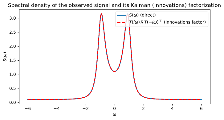
The two curves coincide to machine precision: the Kalman filter has factored the rational spectral density \(S(\omega)\) into \(T(i\omega)\, R\, T(-i\omega)^\top\), with \(T(s)\) the minimum-phase factor. The resonant peak near \(\omega = w_0 = 1\) is the oscillator’s natural frequency; the additive floor \(R\) is the white measurement noise.
(d) The continuous-time linear regulator#
The same matrices now appear in a control problem. Let the state obey the controlled linear system
where \(u(t)\) is an \(m \times 1\) control and \(B\) is \(n \times m\). Choose the control path to minimize the quadratic objective
which penalizes deviations of the state (through \(Q\)) and the use of control (through \(R\)). Let \(V(x)\) be the optimal value of the problem started from \(x\). The principle of optimality gives the Hamilton–Jacobi–Bellman equation
where \(V_x\) is the gradient of \(V\). Guided by the quadratic objective, conjecture a quadratic value function \(V(x) = x^\top P\, x\) with \(P \succeq 0\) symmetric, so \(V_x = 2P x\). The inner minimization over \(u\) is a quadratic with first-order condition \(2 R u + 2 B^\top P x = 0\), giving the optimal feedback law
Substituting \(u = -F x\) back into (97) and requiring the result to hold for all \(x\) yields the control algebraic Riccati equation
The optimally controlled system \(\dot x = (A - BF)\, x\) is stable. The cell below solves the regulator for the same \((A, B)\), penalizing the observed position.
# Linear regulator for the same (A, B): penalize position^2 (= x' C'C x) and control effort.
Q  = C.T @ C
Rc = np.array([[1.0]])

P = solve_continuous_are(A, B, Q, Rc)        # solves A'P + PA - P B Rc^{-1} B'P + Q = 0
F = np.linalg.inv(Rc) @ B.T @ P              # optimal feedback gain, u = -F x

print("value-function matrix P =\n", np.round(P, 4))
print("feedback gain F =", F.ravel().round(4))
print("closed-loop poles eig(A - B F) =", np.linalg.eigvals(A - B @ F).round(4))
value-function matrix P =
 [[0.9417 0.4142]
 [0.4142 0.4902]]
feedback gain F = [0.4142 0.4902]
closed-loop poles eig(A - B F) = [-0.5451+1.0569j -0.5451-1.0569j]
(e) Duality of filtering and control#
Place the two Riccati equations side by side:
They are the same equation under the substitution discovered by Kalman:
Regulator (control) |
Filter (estimation) |
|---|---|
\(A\) |
\(A^\top\) |
control input matrix \(B\) |
observation matrix \(C^\top\) |
state-cost \(Q\) |
process-noise covariance \(BB^\top\) |
control-cost \(R\) |
measurement-noise covariance \(R\) |
value matrix \(P\) (cost-to-go) |
error covariance \(\Sigma\) |
feedback gain \(F = R^{-1}B^\top P\) |
Kalman gain \(K^\top = R^{-1} C\, \Sigma\) |
Replacing \((A, B, Q, R)\) in the regulator equation by the dual data \((A^\top, C^\top, BB^\top, R)\) turns it into the filter equation, with \(P \mapsto \Sigma\) and \(F \mapsto K^\top\). The substitution is an exact mirror: the regulator runs backward in time from a terminal condition, while the filter runs forward from an initial condition, and the duality is the formal expression of that time reversal. Read economically, the cost-to-go of an optimally controlled system coincides with the forecast-error covariance of the dual estimation problem.
One algorithm therefore serves both problems, as does one body of theorems on existence, uniqueness, and stability of the Riccati solution. Indeed in Section (c) we already solved the filter Riccati equation by calling a regulator Riccati solver on transposed data. The next cell makes the correspondence explicit by recovering \(\Sigma\) and \(K\) from the regulator solver applied to the dual data.
# Duality check: solve the regulator CARE on the DUAL data (A', C', BB', R).
# Its value matrix must equal the filter covariance Σ, and its gain must equal K'.
P_dual = solve_continuous_are(A.T, C.T, B @ B.T, R)
F_dual = np.linalg.inv(R) @ C @ P_dual          # = R^{-1} C Σ = K'

print("‖P_dual - Σ‖  =", np.linalg.norm(P_dual - Sigma))
print("‖F_dual - K'‖ =", np.linalg.norm(F_dual - K.T))
print("duality holds:", np.allclose(P_dual, Sigma) and np.allclose(F_dual, K.T))
‖P_dual - Σ‖  = 0.0
‖F_dual - K'‖ = 0.0
duality holds: True
The match is exact: the value matrix of the dual regulator problem is the filter error covariance, and its feedback gain is the transposed Kalman gain. The white innovation \(\eta\) that the filter produces has no predictable increment. It is the locally unpredictable building block of 13. Locally Unpredictable Stochastic Processes.
(f) The innovation, and whether an econometrician can find it#
The innovation \(\eta\) of (90) is the object that Part II is about.
The filter constructed here is a continuous-time filter: it conditions on the entire history \(\{y(s),\ s \leq t\}\), observed without gaps. Under that conditioning \(\eta\) is fundamental, and the innovations representation (91) is a genuine Wold representation with the Kalman gain \(K\) playing the part of the moving-average kernel. An agent inside the model who watches \(y\) continuously sees exactly \(\eta\); it is that agent’s news.
An econometrician with quarterly data does not see \(\eta\). What such an observer can construct is the one-step-ahead error in forecasting \(y_t\) from \(y_{t-1}, y_{t-2}, \ldots\), a discrete-time innovation formed by projecting on a strictly coarser information set. The two objects need not be close, and the relation between them is precisely the subject of 18. Time Aggregation, which writes the discrete innovation as \(a_t = \int_0^\infty f(\tau) w(t-\tau)\, d\tau\) and asks when the kernel \(f\) is concentrated on the last sampling interval, and of 23. Temporal Aggregation of Economic Time Series, which decomposes the discrete innovation exactly as
the second term being the error one makes in recovering the continuous-time forecast from sampled data. The Riccati equation of this chapter tells us what the continuous innovation is; those chapters tell us how much of it survives the passage to discrete data. The answer, in general, is: not all of it, and the shortfall is governed by the behaviour of the kernel at the origin, the condition of 13. Locally Unpredictable Stochastic Processes.
Exercises#
import numpy as np
from scipy.linalg import solve_continuous_are
import matplotlib.pyplot as plt
Exercise 17
The \((A, B, C, D)\) parameterization. Replace the observation equation (83) by
so that the measurement noise is parameterized by its volatility matrix \(D\) and has covariance \(R = DD^\top\).
(a) Show that the steady-state error covariance now solves
and explain why \(DD^\top\) must be nonsingular for the filter to be well posed, so that every component of the observation carries some independent measurement noise.
(b) For the oscillator of the text, take \(D = 0.4\) (a scalar, so \(C\) is \(1 \times 2\)) and verify numerically that the resulting \(\Sigma\) and \(K\) are exactly those obtained with \(R = DD^\top = 0.16\). Confirm that the filter depends on \(D\) only through \(DD^\top\).
Solution to Exercise 17
(a) With \(dy = C x\, dt + D\, dV\) the measurement-noise increment \(D\, dV\) has covariance \(E\, (D\, dV)(D\, dV)^\top = DD^\top dt\). Every place that \(R\) entered the derivation of the filter it entered as the measurement-noise covariance, so the algebraic Riccati equation (89) and gain hold verbatim with \(R\) replaced by \(DD^\top\). The inverse \((DD^\top)^{-1}\) appears in both the Riccati equation and the gain; it exists iff \(DD^\top\) has full rank, i.e. iff \(D\) has full row rank. A direction in observation space with no noise (a zero row of \(D\)) would let the filter extract a noiseless linear combination of the state and drive the corresponding error variance to zero, making \(C^\top (DD^\top)^{-1} C\) unbounded. The filtering problem is then singular, and one must reduce it before the standard CARE applies.
(b) The construction below confirms the filter sees only \(DD^\top\):
w0, zeta, sigma = 1.0, 0.3, 1.0
A = np.array([[0.0, 1.0], [-w0**2, -2*zeta*w0]])
B = np.array([[0.0], [sigma]])
C = np.array([[1.0, 0.0]])

D = np.array([[0.4]])            # measurement volatility
Rdd = D @ D.T                    # = 0.16

Sigma_D = solve_continuous_are(A.T, C.T, B @ B.T, Rdd)
K_D = Sigma_D @ C.T @ np.linalg.inv(Rdd)

# Compare with passing the covariance R = 0.16 directly.
Sigma_R = solve_continuous_are(A.T, C.T, B @ B.T, np.array([[0.16]]))

print("Σ from D    =\n", np.round(Sigma_D, 6))
print("Σ from R=DD' identical:", np.allclose(Sigma_D, Sigma_R))
print("Kalman gain K =", K_D.ravel().round(4))
Σ from D    =
 [[0.213639 0.14263 ]
 [0.14263  0.489662]]
Σ from R=DD' identical: True
Kalman gain K = [1.3352 0.8914]
Exercise 18
A scalar signal observed in noise. Let the state be the Ornstein–Uhlenbeck process of Chapter 7, observed in additive white noise:
with \(a, b > 0\) and \(r > 0\) (here \(A = -a\), \(B = b\), \(C = 1\), \(R = r\)).
(a) The scalar algebraic Riccati equation is \(-2a\Sigma + b^2 - \Sigma^2/r = 0\). Solve it for the steady-state error variance \(\Sigma\), and show that the steady-state filter pole is
Interpret the two limits \(r \to 0\) (precise observations) and \(r \to \infty\) (uninformative observations).
(b) Verify the closed form against solve_continuous_are, then simulate the system and the
steady-state filter with Euler–Maruyama and check that the realized filtering-error variance
matches \(\Sigma\).
Solution to Exercise 18
(a) Multiplying \(-2a\Sigma + b^2 - \Sigma^2/r = 0\) by \(r\) gives \(\Sigma^2 + 2 a r\, \Sigma - b^2 r = 0\), whose positive root is
The gain is \(K = \Sigma/r\), and the filter pole is \(-a - \Sigma/r = -a - \big(-a + \sqrt{a^2 + b^2/r}\big) = -\sqrt{a^2 + b^2/r}\). As \(r \to 0\) the observations are nearly perfect, the pole \(\to -\infty\), and the estimate tracks the state almost instantly; as \(r \to \infty\) the observations are useless, the pole \(\to -a\), and the filter falls back on the prior dynamics of the Ornstein–Uhlenbeck state. This is the state-space echo of the Wiener–Kolmogorov forecast (65) of the AR(1) process: the more informative the data, the faster the filter mean-reverts to the truth.
a, b, r = 1.0, 0.7, 0.05

Sigma = -a*r + np.sqrt(a**2 * r**2 + b**2 * r)      # closed form
K = Sigma / r
pole = -np.sqrt(a**2 + b**2 / r)

# check against the general solver
A1, B1, C1, R1 = np.array([[-a]]), np.array([[b]]), np.array([[1.0]]), np.array([[r]])
Sig_solver = solve_continuous_are(A1.T, C1.T, B1 @ B1.T, R1)[0, 0]

print(f"Σ closed form = {Sigma:.6f},  solver = {Sig_solver:.6f}")
print(f"Kalman gain K = {K:.4f},  filter pole = {pole:.4f}  (= -a - K = {-a-K:.4f})")
Σ closed form = 0.114317,  solver = 0.114317
Kalman gain K = 2.2863,  filter pole = -3.2863  (= -a - K = -3.2863)
(b) Simulate state, observation increments, and the steady-state filter on a fine grid:
rng = np.random.default_rng(0)
dt, T = 0.001, 4000.0
N = int(T / dt)

x = 0.0          # true state
xh = 0.0         # filter estimate
errs = np.empty(N)
sb, sv = b*np.sqrt(dt), np.sqrt(r)*np.sqrt(dt)
for k in range(N):
    dW = rng.normal() * np.sqrt(dt)
    dy = x*dt + sv*rng.normal()           # observation increment over [t, t+dt]
    xh = xh - a*xh*dt + K*(dy - xh*dt)     # steady-state Kalman-Bucy update
    x  = x  - a*x*dt + b*dW                # true state update
    errs[k] = x - xh

burn = int(200 / dt)
print(f"realized error variance = {errs[burn:].var():.5f},   Σ = {Sigma:.5f}")
realized error variance = 0.11301, Σ = 0.11432
fig, ax = plt.subplots(figsize=(9, 3.5))
tt = np.arange(burn, burn + int(20/dt)) * dt
ax.plot(tt, errs[burn:burn + int(20/dt)], lw=0.7)
ax.axhline(np.sqrt(Sigma), color='k', ls='--', lw=1, label=r'$\pm\sqrt{\Sigma}$')
ax.axhline(-np.sqrt(Sigma), color='k', ls='--', lw=1)
ax.set_xlabel('$t$'); ax.set_ylabel(r'$x(t)-\hat x(t)$')
ax.set_title('Filtering error and its steady-state standard deviation')
ax.legend(); plt.show()
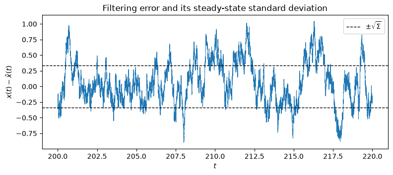
The realized error variance matches the Riccati value \(\Sigma\), and the error stays within the \(\pm\sqrt{\Sigma}\) band predicted by the steady-state filter.