18. Time Aggregation#
by Lars Peter Hansen and Thomas J. Sargent
Note
This chapter reproduces Section 2 of Hansen and Sargent, Two Difficulties in Interpreting Vector Autoregressions. The original equation, figure, and table numbering of that section is retained. References to “the previous section” and to equation \((7)\) point to the surrounding parts of the original paper, which are not reproduced here.
Consider a linear economic model that is formulated in continuous time, and which can be represented as
where \(z(t)\) is an \((n \times 1)\) vector stochastic process, \(w(t)\) is an \((m \times 1)\) vector white noise with \(Ew(t)w(t-s)^T = \delta(t-s)I\), \(\delta\) is the Dirac delta generalized function, and \(p(\tau)\) is an \((n \times m)\) matrix function that satisfies \(\int_0^\infty \operatorname{trace} p(\tau)p(\tau)^T\, d\tau < +\infty\). We let \(P(s) = \int_0^\infty e^{-s\tau} p(\tau)\, d\tau\), i.e., \(P(s)\) is the Laplace transform of \(p(\tau)\). Sometimes we shall find it convenient to write (124) in operator notation
where \(D\) is the derivative operator. We shall assume that \(\det P(s)\) has no zeroes in the right half of the complex plane. This guarantees that square integrable functionals of \((z(t-s),\ s \geq 0)\) and of \((w(t-s),\ s \geq 0)\) span the same linear space, and is equivalent to specifying that (124) is a Wold representation for \(z(t)\).
A variety of continuous time stochastic linear rational expectations models have equilibria that assume the form of the representations (124) or (125); the methods of 16. Faster Methods for Solving Recursive Linear Models of Dynamic Economies compute them. Hansen and Sargent (1981d) provide some examples. The continuous-to-discrete sampling map exploited throughout this chapter is the same one analyzed from the identification side by 21. Inferring a Continuous-Time System from Discrete-Time Data: An Appreciation of A. W. Phillips (1959) and 22. The Dimensionality of the Aliasing Problem in Models with Rational Spectral Densities, while the closely related Cagan inverse-optimal-predictor construction is taken up in 20. Aggregation Over Time and the Inverse Optimal Predictor Problem for Adaptive Expectations in Continuous Time. In these examples, the continuous time white noises \(w(t)\) often have interpretations as innovations in the uncontrollable processes that agents care about forecasting, and which stochastically drive the model. These include processes that are imagined to be observable to both the econometrician and the private agent (e.g., various relative prices and quantities) and also those which are observable to private agents but are hidden from the econometrician (e.g., random disturbances to technologies, preferences, and maybe even particular factors of production such as effort or capital of specific kinds). The \(w(t)\) process is economically interpretable as the continuous time innovation to private agents, because a forecast error of the variables in the model over any horizon \(t+\tau\) which the private agents are assumed to make at \(t\) can be expressed as a weighted sum of \(w(s)\), \(t < s \leq t + \tau\). Thus, to private agents the \(w(t)\) process represents news or surprises.
In rational expectations models, typically there are extensive restrictions across the rows of \(P(D)\). In general these restrictions leave open the possibility that the current and lagged values of the \(w(t)\) process span a larger linear space than do current and lagged values of the \(z(t)\) process. This outcome can possibly occur even if the dimension \(m\) of the \(w(t)\) process is less than or equal to the dimension \(n\) of the \(z(t)\) process. This is the continuous time version of the phenomenon that we treated for discrete time in the previous section. In the present section, we ignore this phenomenon, by assuming that \(\det P(s)\) has no zeroes in the right half of the complex plane.
For this continuous time specification, there exists a discrete time moving-average representation
where \(C(L)\) is an infinite order, \((n \times n)\) polynomial in the lag operator \(L\), where \(a_t\) is a vector white noise with \(Ea_t a_t^T = W\), and where \(a_t = z_t - \hat{E}[z_t \mid z_{t-1}, \ldots]\). The operator \(C(L)\) and the positive semi-definite matrix \(W\) solve the following equation, subject to the side condition that the zeroes of \(\det C(z)\) do not lie inside the unit circle:[1]
The right side of (127) is the folding of the continuous time spectral density onto the discrete-frequency band. It is the matrix counterpart of the folding formula (123) of 17. Discrete Sampling: The Folding Formula, and the source of the aliasing that the rest of this chapter traces.
When \(z_t\) has a discrete time autoregressive representation, the discrete time innovations \(a_t\) are related to the \(w(t)\) process by the formula
or
where we have defined \(V(L) = C(L)^{-1} = \sum_{j=0}^{\infty} V_j L^j\), \(V_0 = I\). Here \(-V_j\) is the \(n \times n\) matrix of coefficients on the \(j^{\text{th}}\) lag in the vector autoregression for \(z\). It follows directly upon writing out (128) that
where[2]
It also follows from (129) and the identity for integer \(t\), \(C(L) a_t = P(D) w_t\), that
Equations (129) and (130) show how the discrete time innovation \(a_t\) in general reflects all past values of the continuous time innovation \(w(t)\).
Analyses of vector autoregressions often proceed by summarizing the shape of \(C(L)\) in various ways, and attempting to interpret that shape. The innovation accounting methods of Sims, based on decomposition \((7)\), are good examples of procedures that summarize the shape of \(C(L)\). From the viewpoint of interpreting discrete time vector autoregressions in terms of the economic forces acting on individual agents, it would be desirable if the discrete time and continuous time moving-average representations were to match up in some simple and interpretable ways. In particular, the following two distinct but related features would be desirable. First, it would be desirable if the discrete time innovations \(a_t\) closely reflected the behavior of \(w(s)\) near \(t\). Probably the most desirable outcome would be if \(a_t\) could be expressed as
so that in (129), \(f(\tau) = 0\) for \(\tau > 1\). In that case, \(a_t\) would be a weighted sum of the continuous time innovations over the unit forecast interval. It would be even more desirable if (132) were to hold with \(f(\tau) = p(\tau)\), for then \(a_t\) would equal the one step ahead forecast error from the continuous time system. Second, assuming a smooth \(p(\tau)\) function, it would be desirable if the discrete time moving-average coefficients \(\{C_0, C_1, C_2, \ldots\}\) resemble a sampled version of the continuous time moving average kernel \(\{p(\tau),\ \tau \geq 0\}\). This is desirable because the pattern of the \(C_j\)’s would then faithfully reflect the response of the system to innovations in continuous time. We shall consider each of these desiderata in turn.
We first study conditions under which \(f(\tau) = 0\) for \(\tau > 1\). Consider the decomposition
This last equality implies that if (132) is to hold it must be the case that
which in turn implies that \(p(\tau) = f(\tau)\) for \(0 \leq \tau \leq 1\). The interpretation of requirement (133) is that the discrete time and continuous time forecasts of \(z(t)\) over a unit time interval coincide.
When condition (132) is met, the link between \(P(D)\) and \(C(L)\) is particularly simple. Using \(f(\tau) = 0\) for \(\tau > 1\), equation (131) becomes
Equation (134) implies that for the particular class of continuous time processes for which \(f(\tau) = 0\) for \(\tau > 1\), the continuous time moving-average coefficients are completely determined by the discrete time moving-average coefficients and the function \(f(\tau)\) defined on the unit interval. The aliasing problem is manifested in this relationship because \(f(\tau)\) cannot be inferred from discrete time data. In the absence of additional restrictions, all functions \(f(\tau)\) that satisfy
are observationally equivalent. Relation (134) also implies that in general, without some more restrictions on \(p(\tau)\), condition (132) does not place any restrictions on the discrete time moving-average coefficients.
However, in many (if not most) applications, it is usual to impose the additional requirement that the continuous time moving-average coefficients be a continuous function of \(\tau\).[3] This requirement together with (134) then imposes a very stringent restriction on the discrete time moving-average representation. In particular, (134) then implies that
where \(f(\tau)\) is now a continuous function on the unit interval. When \(w(t)\) and \(z(t)\) have the same dimension (\(m = n\)) and \(f(0)\) is nonsingular, relation (135) implies that
and
This implies that if (132) is to hold, the discrete time process must have a first order autoregressive representation. We have therefore established that condition (132) and the continuity requirement on \(p(\tau)\) substantially restrict not only the admissible continuous time moving-average coefficients but the admissible discrete time moving-average coefficients as well.
Thus, with a continuous \(p(\tau)\) function, in general, relation (132) does not hold. Instead, \(a_t\) given by (129) is a function of all current and past \(w(t)\)’s, a function whose nature can pose problems in several interrelated ways for interpreting \(a_t\) in terms of the continuous time noises \(w(t)\) that are imagined to impinge on agents in the model. First, as in the discrete time case, the process \(w(t)\) need not be fundamental for \(z(t)\) in continuous time. Second, the matrix function \(f(\tau)\) in (129) is not usually diagonal, so that each component of \(a_t\) in general is a function of all of the components of \(w(t)\). This is a version of what Geweke (1978) has characterized as “contamination,” which occurs in the context of the aggregation over time of several interrelated distributed lags. It is also related to the well-known phenomenon that aggregation over time generally leads to Granger-causality of discrete sampled \(y\) to \(x\) even when \(y\) fails to Granger-cause \(x\) in continuous time. Third, the matrix function \(f(\tau)\) in (128) in general is nonzero for all values of \(\tau > 0\), so that \(a_t\) in general depends on values of \(w(t-\tau)\) in the remote past.
We now turn to our second desideratum, namely that the sequence \(\{C_j\}_{j=0}^{\infty}\) resemble a sampled version of the function \(p(\tau)\). For studying this matter, we set \(m = n\), because we are interested in studying circumstances under which \(\{C_j\}\) fails to reflect \(p(\tau)\) even when the number of white noises \(n\) in \(a_t\) equals the number \(m\) in \(w(t)\). We can represent most of the issues here with a univariate example, and so set \(m = n = 1\) in most of our discussion. It is also convenient to study the case in which \(z_t\) has a rational spectral density in continuous time, the class introduced in 8. Spectral Densities and generated by the linear stochastic differential equations of 11. Linear Stochastic Differential Equations, whose sum-of-exponentials kernel \(p(\tau) = \sum_j \delta_j e^{\lambda_j \tau}\) reappears below. Thus we assume that
where \(z_t\) is a scalar stochastic process, and \(\theta(s) = (s - \lambda_1)(s - \lambda_2) \cdots (s - \lambda_r)\), \(\psi(s) = \psi_0 + \psi_1 s + \cdots + \psi_{r-1} s^{r-1}\). We assume that the real parts of \(\lambda_1, \ldots, \lambda_r\), which are the zeroes of \(\theta(s)\), are less than zero, but that the real parts of the zeroes of \(\psi(s)\) are unrestricted. Only if the real parts of the zeroes of \(\psi(s)\) are less than zero do current and past values of \(z(t)\) and \(w(t)\) span the same linear space. If any zeroes of \(\psi(s)\) have real parts that exceed zero, then current and lagged \(w(t)\) span a larger space than do current and lagged \(z(t)\). The above equation can be expressed as
where \(P(D) = \psi(D)/\theta(D)\). A partial fraction representation of \(P(D)\) is
where
We therefore have
Thus, the weighting function \(p(\tau)\) in the continuous time moving-average representation is a sum of \(r\) exponentially decaying functions. Our object will now be to get an analogous expression to (140) for the discrete time coefficients \(C_k\).
It is known that the discrete time process \(z_t\) implied by (136) is an \(r^{\text{th}}\) order autoregressive, \((r-1)\) order moving average process. Let this be \(z_t = \frac{c(L)}{d(L)} a_t\) where \(c(L) = \sum_{j=0}^{r-1} c_j L^j\), \(d(L) = \sum_{j=0}^{r} d_j L^j\). To find this representation, we must use (127). A.W. Phillips (1959) and Hansen and Sargent (1983b) show that for the process (136), the term on the right side of (127) can be represented
where
Letting \(z = e^{-i\omega}\), to find the required mixed moving-average autoregressive representation we must solve
subject to the condition that the zeroes of \(c(z)\) and \(d(z)\) all lie outside the unit circle. The term on the right side of (141) can be expressed as
where \(\alpha_j \equiv e^{\lambda_j}\). Note that \(|\alpha_j| < 1\) by virtue of the assumption that \(\operatorname{real}(\lambda_j) < 0\). Thus, the denominator is already factored as required, so that
The numerator must be factored to find \(c(z)\). Standard procedures to find the zeroes of scalar polynomials can be used to achieve this factorization, as described by Hansen and Sargent (1981a).
Thus we have that
Proceeding in a similar fashion as we did for the continuous time moving-average representation, we can find a partial fraction representation for \(C(L)\), namely
where
Recalling that \(\alpha_j = e^{\lambda_j}\), equation (145) implies that
Collecting and comparing the key results, we have that
Equations (140) and (147) imply that \(C_k\) will be (proportional to) a sampled version of \(p(\tau)\) if and only if \(\gamma_j/\delta_j = \gamma_1/\delta_1\) for all \(j = 2, \ldots, r\). It can be shown directly by using (140) and (147) in (130) and (131) that this condition will not be met for any \(r \geq 2\). Thus, only if \(z(t)\) is a first-order autoregressive process does \(C_k\) turn out to be a sampled version of \(p(\tau)\).
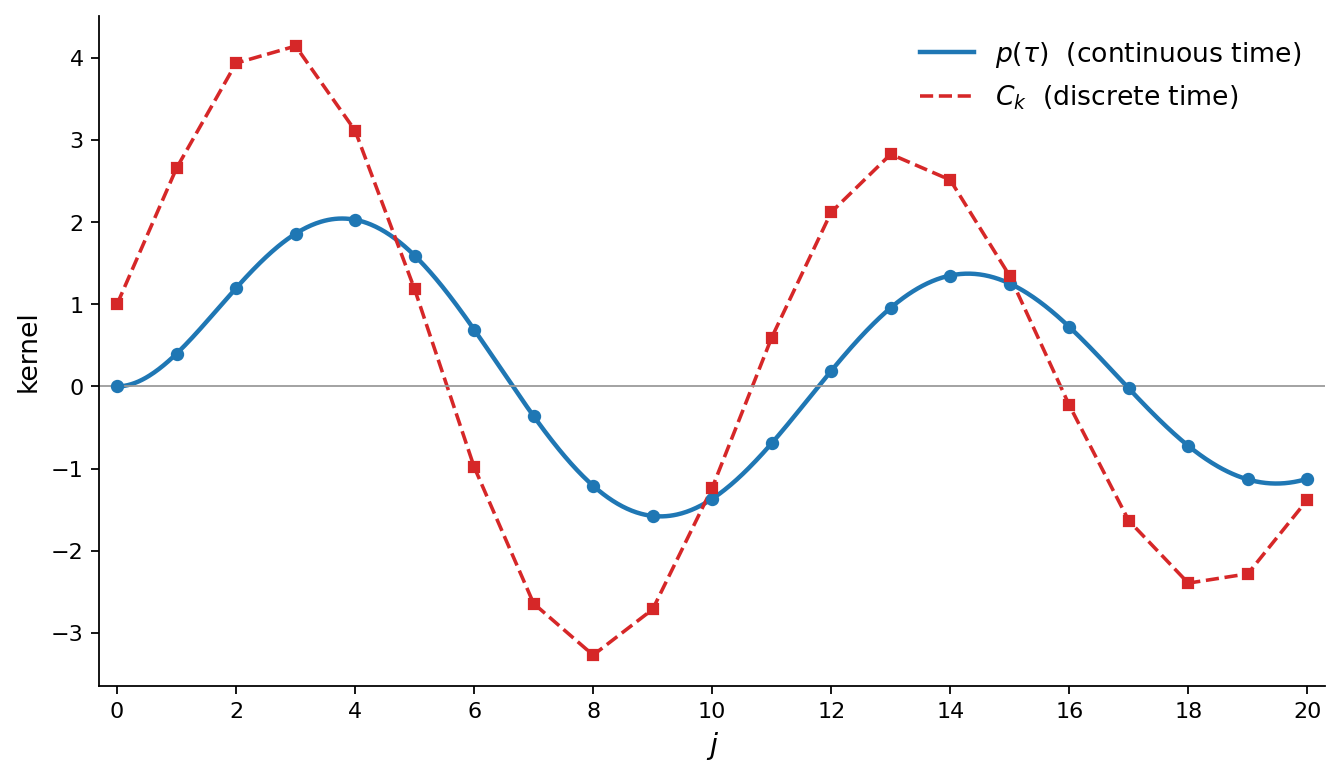
Fig. 5 Figure 5. Continuous time and discrete time moving-average kernels for the example of Table 1. The solid curve is the continuous time kernel \(p(\tau) = \sum_{j=1}^{3} \delta_j e^{\lambda_j \tau}\) (markers show its integer samples \(p(j)\)); the dashed line is the discrete time kernel \(C_k\). The two kernels share the roots \(\lambda_j\) but have different residues, so \(C_k\) is not a sampled version of \(p(\tau)\).#
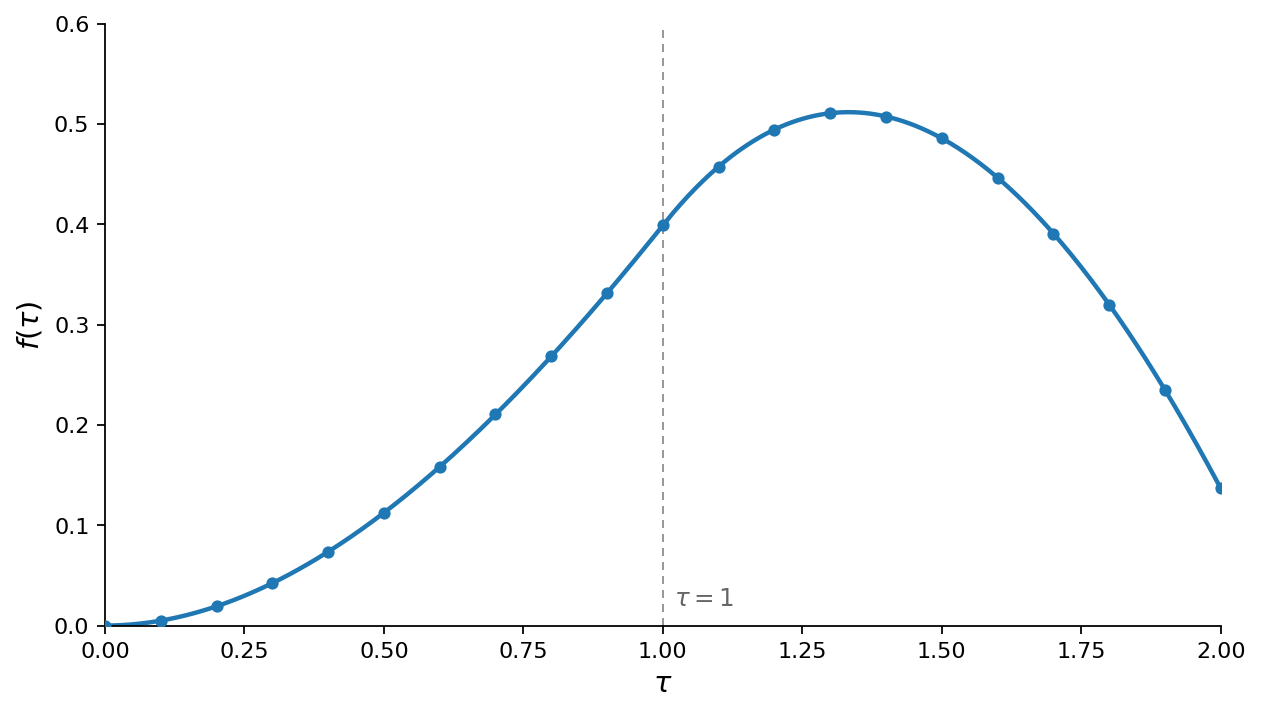
Fig. 6 Figure 6. The aggregation kernel \(f(\tau)\) of (130) for the example of Table 1. On \([0,1]\) it coincides with \(p(\tau)\); it does not vanish for \(\tau > 1\), and is in fact larger in absolute value over most of \([1,2]\) than over \([0,1]\), a consequence of the system being third order rather than first order in continuous time.#
Table 1 and Figure 5 present a numerical example that illustrates the preceeding ideas. For the univariate process \((D^3 + .6D^2 + .4D + .2)\, z(t) = w(t)\), we have calculated \(p(\tau)\), \(f(\tau)\), \(c(L)\), \(d(L)\), \(C(L) = c(L)/d(L)\), \(\delta_j\), \(\gamma_j\) for \(j = 1, 2, 3\). In this example, we have that \(\gamma_j/\gamma_1 \neq \delta_j/\delta_1\) for \(j \geq 2\), so that the shapes of the moving averages in continuous and discrete time, \(p(\tau)\) and \(C_k\), respectively, are different. We plot \(C_k\) and \(p(\tau)\) for integer values of \(\tau\) in Figure 5. We also plot \(f(\tau)\) in Figure 6. Notice that \(f(\tau) \neq 0\) for some \(\tau\)’s greater than 1. In particular, notice that \(f(\tau)\) is larger in absolute value over most of the interval \([1, 2]\) than it is over the interval \([0, 1]\). The failure of \(f(\tau)\) to be concentrated on \([0, 1]\) and the failure of \(C_k\) to resemble a sampled version of \(p(\tau)\) are both consequences of the fact that this is a third order autoregressive system in continuous time, rather than a first order one.
The preceding results and the example generalize readily to the case of a vector stochastic process \(z_t\). Matrix versions of (140) and (147) hold, where the \(\lambda_j\)’s are the zeroes of \(\det \theta(s)\) and the \(\delta_j\)’s and the \(\gamma_j\)’s are \((n \times n)\) matrices given by (139) and (146).
Table 1. An Example of Aggregation Over Time
The continuous time process is the third-order system
whose characteristic roots \(\lambda_j\) (the zeroes of \(\theta(s)\)) are
The implied discrete time mixed moving-average autoregressive representation \(z_t = \big(c(L)/d(L)\big)\, a_t\) has
The zeroes of the numerator spectral factor \(c(z) = 1 + .4800z + .0192z^2\) are real and equal to \(-2.294\) and \(-22.706\); they lie outside the unit circle, as the side condition on (141) requires. (Equivalently, writing \(c(z) = \prod_k (1 - \beta_k z)\), the reciprocal roots are \(\beta_1 = -.4359\) and \(\beta_2 = -.0441\), both of modulus less than one.)
The residues of the continuous time kernel \(p(\tau) = \sum_j \delta_j e^{\lambda_j \tau}\) and of the discrete time kernel \(C_k = \sum_j \gamma_j e^{\lambda_j k}\) are reported below. Because \(\gamma_j/\gamma_1 \neq \delta_j/\delta_1\) for \(j \geq 2\), the discrete time kernel \(C_k\) is not a sampled version of \(p(\tau)\) (Fig. 5).
\(j\) |
\(\operatorname{Re}\delta_j\) |
\(\operatorname{Im}\delta_j\) |
\(\delta_j/\delta_1\) |
\(\operatorname{Re}\gamma_j\) |
\(\operatorname{Im}\gamma_j\) |
\(\gamma_j/\gamma_1\) |
|---|---|---|---|---|---|---|
1 |
\(1.5831\) |
\(0\) |
\(1.000\) |
\(1.7984\) |
\(0\) |
\(1.000\) |
2 |
\(-.7915\) |
\(.6701\) |
\(-.500 + .423\,i\) |
\(-.3992\) |
\(2.0310\) |
\(-.222 + 1.129\,i\) |
3 |
\(-.7915\) |
\(-.6701\) |
\(-.500 - .423\,i\) |
\(-.3992\) |
\(-2.0310\) |
\(-.222 - 1.129\,i\) |
Panel A. The kernels at integer lags \(k = 0, 1, \ldots, 20\) (plotted in Fig. 5). The column \(f(k)\) shows how rapidly the aggregation kernel \(f\) of (130) decays once \(\tau\) exceeds \(1\).
\(k\) |
\(p(k)\) |
\(C_k\) |
\(f(k)\) |
|---|---|---|---|
0 |
\(0\) |
\(1.000000\) |
\(0\) |
1 |
\(.398987\) |
\(2.657971\) |
\(.398987\) |
2 |
\(1.197125\) |
\(3.935901\) |
\(.136629\) |
3 |
\(1.860267\) |
\(4.144677\) |
\(-.073263\) |
4 |
\(2.029242\) |
\(3.116763\) |
\(.032542\) |
5 |
\(1.593759\) |
\(1.188521\) |
\(-.014212\) |
6 |
\(.692895\) |
\(-.972014\) |
\(.006197\) |
7 |
\(-.361072\) |
\(-2.631591\) |
\(-.002701\) |
8 |
\(-1.208944\) |
\(-3.259333\) |
\(.001178\) |
9 |
\(-1.576723\) |
\(-2.705194\) |
\(-.000513\) |
10 |
\(-1.368770\) |
\(-1.233866\) |
\(.000224\) |
11 |
\(-.692635\) |
\(.588609\) |
\(-.000098\) |
12 |
\(.188765\) |
\(2.107332\) |
\(.000043\) |
13 |
\(.956663\) |
\(2.810459\) |
\(-.000019\) |
14 |
\(1.350008\) |
\(2.498675\) |
\(.000008\) |
15 |
\(1.252755\) |
\(1.336741\) |
\(-.000004\) |
16 |
\(.725963\) |
\(-.224260\) |
\(.000002\) |
17 |
\(-.020340\) |
\(-1.619749\) |
\(-.000001\) |
18 |
\(-.722582\) |
\(-2.374213\) |
\(.000000\) |
19 |
\(-1.131496\) |
\(-2.261452\) |
\(-.000000\) |
20 |
\(-1.124345\) |
\(-1.369232\) |
\(.000000\) |
Panel B. The aggregation kernel \(f(\tau)\) on \([0,2]\) (plotted in Fig. 6). On \([0,1]\), \(f(\tau) = p(\tau)\); the two diverge for \(\tau > 1\).
\(\tau\) |
\(f(\tau)\) |
\(p(\tau)\) |
|---|---|---|
\(.0\) |
\(0\) |
\(0\) |
\(.1\) |
\(.004900\) |
\(.004900\) |
\(.2\) |
\(.019198\) |
\(.019198\) |
\(.3\) |
\(.042288\) |
\(.042288\) |
\(.4\) |
\(.073563\) |
\(.073563\) |
\(.5\) |
\(.112414\) |
\(.112414\) |
\(.6\) |
\(.158231\) |
\(.158231\) |
\(.7\) |
\(.210404\) |
\(.210404\) |
\(.8\) |
\(.268324\) |
\(.268324\) |
\(.9\) |
\(.331386\) |
\(.331386\) |
\(1.0\) |
\(.398987\) |
\(.398987\) |
\(1.1\) |
\(.457506\) |
\(.470529\) |
\(1.2\) |
\(.494395\) |
\(.545421\) |
\(1.3\) |
\(.510679\) |
\(.623079\) |
\(1.4\) |
\(.507397\) |
\(.702926\) |
\(1.5\) |
\(.485602\) |
\(.784396\) |
\(1.6\) |
\(.446360\) |
\(.866935\) |
\(1.7\) |
\(.390751\) |
\(.949999\) |
\(1.8\) |
\(.319860\) |
\(1.033059\) |
\(1.9\) |
\(.234786\) |
\(1.115601\) |
\(2.0\) |
\(.136629\) |
\(1.197125\) |
(a) Locally Unpredictable Processes and Linear Quadratic Models#
Note
This section reproves, in the notation of the original paper, results that earlier chapters established. Its condition \(p(0) = p'(0) = \cdots = p^{(j-1)}(0) = 0\) for \(j\)-fold mean square differentiability is Theorem 12 of 9. Characterizations of Mean Square Differentiability and Mean Square Continuity. Its definition (148) of local unpredictability is Definition 10 of 13. Locally Unpredictable Stochastic Processes. Its computation \(g(0) = \lim_{s\to\infty} sG(s) = P(-\rho)\) is the calculation performed there. The citations to “Sargent (1983)” in the text below are the original paper’s; within this book they point to Chapters 9 and 13. Two things here are new. Equation (149) bridges local unpredictability and the behaviour of the sampled forecast error as the sampling interval shrinks. And adjustment-cost models smooth \(x^*(t)\) back into mean square differentiability, so appealing to that limit does not escape the difficulty.
The stochastic process \(z(t)\) in Table 1 is mean square differentiable,[4] as evidenced by the fact that \(p(0) = 0\). A stochastic process of the form (124) can be shown to be \(j\) times mean square differentiable if \(p(0) = p'(0) = p''(0) = \ldots = p^{(j-1)}(0) = 0\) (see Sargent (1983) for a proof). Consequently, the process \((D^3 + .6D^2 + .4D + .2)z(t) = w(t)\) can be verified to be twice (but not three times) mean square differentiable. It is the smoothness and proximity to zero near \(\tau = 0\) of \(p(\tau)\) that makes it difficult for \(C_j\) to resemble a sampled version of \(p(\tau)\), and that makes \(a(t)\) a poor estimator of \(\int_0^1 p(\tau)w(t-\tau)\, d\tau\).
Sims (1984) argued that there is a class of economic variables that are best modeled as failing to be mean square differentiable. For these processes, \(p(0) \neq 0\). Processes of the form (124) in which \(p(0) \neq 0\) are said to be locally unpredictable (the subject of 13. Locally Unpredictable Stochastic Processes) because if \(p(0) \neq 0\), then
Here \(\hat{E}_t\) is the linear least squares projection operator, conditioned on \(\{x(t-s),\ s \geq 0\}\). Now condition (148) can readily be shown to imply that
In (149), \(\hat{E}_t x(t+\delta)\) is the linear least squares projection of \(x(t+\delta)\) conditioned on \((x(t-s),\ s \geq 0)\), while \(\hat{E}(x(t+\delta) \mid x(t), x(t-\delta), \ldots)\) is the projection of \(x(t+\delta)\) on the discrete time sample \(x(t), x(t-\delta), \ldots\) Condition (149) holds for any locally unpredictable process, and states that for small enough sampling interval \(\delta\), the \(\delta\)-ahead projection error from the continuous time process is close in the mean square error sense to the \(\delta\)-ahead projection error from the \(\delta\)-discrete time data. Thus, when \(p(0) \neq 0\), for small enough \(\delta\), the innovation \(a_t\) in the \(\delta\)-counterpart to (144) is arbitrarily close to \(\int_0^{\delta} p(s)w(t-s)\, ds\) in the mean square sense.
Now suppose that \(z(t)\) is given by (124), with \(p(0) = 0\), so that \(z(t)\) is mean square differentiable. Following Sims (1984), suppose that the economist is interested in studying the expectational variable \(x^*(t)\) given by
where \(\rho < 0\). Hansen and Sargent (1981d) showed that
where \(P(s) = \int_0^\infty e^{-\tau s} p(\tau)\, d\tau\) is the Laplace transform of \(p(\tau)\). Now if \(G(s)\) is the Laplace transform of \(g(\tau)\), with support \([0, \infty)\), the initial value theorem for Laplace transforms states that
Using the initial value theorem together with (151), we find that
(We know that \(P(-\rho) \neq 0\) because \(P(s)\) is assumed to have no zeroes in the right half of the complex plane by the assumption that \(p(\tau)\) is the kernel associated with a Wold representation for \(z(t)\).) Therefore, even if \(p(0) = 0\), \(g(0) \neq 0\), so that the geometric expectational variable \(x^*(t)\) fails to be mean square differentiable and therefore is locally unpredictable. For such expectational variables, (149) holds. Therefore, for such variables, for small enough sampling interval \(\delta\), the discrete time innovation \(a(t)\) corresponding to (144) is close to \(\int_0^{\delta} g(s)w(t-s)\, ds\) in the mean squared sense. Here \(g\), not \(p\), is the relevant kernel, since it is \(x^*\) rather than \(z\) that is being sampled, and it is \(g(0) = P(-\rho) \neq 0\) that makes the approximation work.
These results imply that for a variable \(x^*(t)\) and sufficiently small sampling interval \(\delta\), the situation is not as bad as is depicted by the example in Table 1. As Sims has pointed out, there are theories of consumption and asset pricing which imply that consumption or asset prices behave like \(x^*(t)\) and are governed by a version of (150). For example, with \(x^*(t)\) being consumption and \(z(t)\) income, (150) is a version of the permanent income theory. Alternatively, with \(x^*(t)\) being a stock price and \(z(t)\) being the dividend process, (150) is a simple version of an asset-pricing formula.
However, there is a wide class of generalized adjustment cost models discussed by Hansen and Sargent (1981a, 1981d) in which observable variables are such smoothed versions of \(x^*(t)\) that they are mean square continuous. In adjustment cost models, decisions are driven by convolutions of \(x^*(t)\), not by \(x^*(t)\) alone. For example, the stochastic Euler equation for a typical quadratic adjustment cost problem is
where \(\rho < 0\) as in (150), so that \(D - \rho\) is a stable operator, or equivalently
since \(-1/(\rho + D)\) applied to \(z\) is precisely the geometric distributed lead \(\int_0^\infty e^{\rho s} z(t+s)\, ds\) of 12. Linear Least Squares Prediction.
Here \(k(t)\) is capital. The solution for capital is then
or
where \(z(t) = \int_0^\infty p(s) w(t-s)\, ds\). Let
and
Then
Using the initial value theorem to calculate \(h(0)\), we have
Thus, \(k(t)\) is mean square differentiable and so is locally predictable. (The convolution integration required to transform \(x^*(t)\) to \(k(t)\) smooths \(k(t)\) relative to \(x^*(t)\).)
More generally, the endogenous dynamics of adjustment cost models typically lead to mean square differentiable endogenous variables, provided that the agent is posited to be facing mean square differentiable forcing processes \((z(t))\). This means that for such models, the difficulties of interpretation that are illustrated in Table 1 cannot be eluded by appealing to an approximation based on the limit (149).
(b) Remedies in Continuous Time Analyses#
The preceding problems of interpretation are results of estimating vector autoregressions while foregoing the imposition of any explicit economic theory in estimation. These problems can be completely overcome if a sufficiently restrictive and reliable dynamic model economy is available to be imposed during estimation. For example, Hansen and Sargent (1980b, 1981d) have described how the function \(p(\tau)\) can be identified and estimated from observations on discrete time data in the context of a wide class of linear rational expectations models. The basic idea is that the rich body of cross-equation restrictions that characterize dynamic linear rational expectations models can be used to identify a unique continuous time model from discrete time data.
If an estimate of \(p(\tau)\) is available, then by using only discrete time data on \(\{z_t\}\), it is even possible to recover an estimate of the one-step prediction error that agents are making in continuous time. This is accomplished by treating the continuous time forecast error as a hidden variable whose covariances with the discrete time process \(\{z_t\}\) are known. Thus, given estimates of \(p(\tau)\), let us define the one-step ahead prediction error from continuous time data as \(e_t^* = \int_0^1 p(\tau) w(t-\tau)\, d\tau\). Then it is straightforward to calculate the following second moments:
We can estimate the projection \(\sum_{j=-m_1}^{m_2} D_j z_{t-j}\) in the projection equation
where \(u_t\) is orthogonal to \(z_{t-j}\) for all \(j = -m_1, \ldots, m_2\). The \(D_j\)’s can be computed from the normal equations
These calculations could be of use if one’s aim were truly to extract and to interpret estimates of the forecast errors made by agents. In continuous time versions of various models, such as those of Lucas (1973) or Barro (1977), agents’ forecasting errors are an important source of impulses, so that it is of interest to have this method for characterizing their stochastic properties and estimating them.
Notes#
## References

```{note}
The citations in the text above are the original paper's, and they carry that paper's letter
suffixes. Hansen and Sargent published several closely related papers in 1980, 1981, and 1983,
and the entries below record the ones the suffixes draw on. Two of the works cited appear in
this book: the geometric distributed lead {eq}`eq-18-2-28` attributed to Hansen and Sargent
(1981d) is derived in {doc}`19_prediction_formulas_continuous_time`, and is the formula
{eq}`eq-12-gen` of {doc}`12_prediction`; the discrete time representation attributed to Hansen
and Sargent (1983b) is the subject of {doc}`22_dimensionality_aliasing_problem`. The citations
to "Sargent (1983)" are to the 1983 class notes that became Chapters 1 through 14 and 17 of
this book; for mean square continuity and differentiability see
{doc}`02_mean_square_continuity_differentiability` and
{doc}`09_characterizations_ms_differentiability`.
Barro, R. J. (1977). Unanticipated Money Growth and Unemployment in the United States. American Economic Review, 67, 101–115.
Christiano, L. (1980). Rational Expectations, Hyperinflation, and the Demand for Money. Manuscript.
Geweke, J. (1978). Temporal Aggregation in the Multiple Regression Model. Econometrica, 46, 643–661.
Hansen, L. P., and T. J. Sargent (1980). Formulating and Estimating Dynamic Linear Rational Expectations Models. Journal of Economic Dynamics and Control, 2, 7–46.
Hansen, L. P., and T. J. Sargent (1981). Linear Rational Expectations Models for Dynamically Interrelated Variables, in R. E. Lucas, Jr., and T. J. Sargent, eds., Rational Expectations and Econometric Practice. Minneapolis: University of Minnesota Press.
Hansen, L. P., and T. J. Sargent (1981). Identification of Continuous Time Rational Expectations Models from Discrete Time Data. Unpublished manuscript. Later published in L. P. Hansen and T. J. Sargent, eds., Rational Expectations Econometrics. Boulder: Westview Press, 1991.
Hansen, L. P., and T. J. Sargent (1982). Continuous Time Models of Control, Prediction, and Rational Expectations.
Hansen, L. P., and T. J. Sargent (1983). Aggregation Over Time and the Inverse Optimal Predictor Problem for Adaptive Expectations in Continuous Time. International Economic Review, 24, 1–20. (Reported in 20. Aggregation Over Time and the Inverse Optimal Predictor Problem for Adaptive Expectations in Continuous Time.)
Hansen, L. P., and T. J. Sargent (1983). The Dimensionality of the Aliasing Problem in Models with Rational Spectral Densities. Econometrica, 51, 377–387. (Reported in 22. The Dimensionality of the Aliasing Problem in Models with Rational Spectral Densities.)
Lucas, R. E., Jr. (1973). Some International Evidence on Output-Inflation Tradeoffs. American Economic Review, 63, 326–334.
Phillips, A. W. (1959). The Estimation of Parameters in Systems of Stochastic Differential Equations. Biometrika, 46, 67–76. (Discussed in 21. Inferring a Continuous-Time System from Discrete-Time Data: An Appreciation of A. W. Phillips (1959).)
Sargent, T. J. (1983). Continuous Time Stochastic Processes. Class notes, University of Minnesota. (Chapters 1 through 14 and 17 of this book.)
Sims, C. A. (1984). Martingale-Like Behavior of Prices and Interest Rates. Discussion paper, University of Minnesota.