5. Stochastic Processes Driven by a Poisson Counting Process

We now study a class of differential equations that are driven by the generalized derivative \(dN/dt\) of a Poisson counting process, the white noise built in 3. The Poisson Counting Process. We can represent the equation that we study formally in three alternative ways.

(19)\[\begin{split}\begin{aligned} (a)\quad \frac{dx}{dt} &= f\bigl(x(t),\, t\bigr) + g\bigl(x(t),\, t\bigr)\ \frac{dN(t)}{dt} \\[4pt] (b)\quad dx &= f\bigl(x(t),\, t\bigr)dt + g\bigl(x(t),\,t\bigr) dN(t) \\[4pt] (c)\quad x(t) &= x(0) + \int_0^t f\bigl(x(s),\, s\bigr) ds + \int_0^t g\bigl(x(s),\, s\bigr) dN(s), \end{aligned}\end{split}\]

with \(x(0)\) given and \(t \geq 0\).

Here \(N(t)\) is a Poisson counting process with rate \(\lambda > 0\), and \(f(x,\, t)\) and \(g(x,\,t)\) are continuous functions. (Add additional regularity conditions.) We now want to define what we mean by a solution to the differential equation (19).

Definition 9

A stochastic process \(x(t)\) is said to be a solution of the stochastic differential equation (19) in the Ito sense if:

(i) on an interval where \(N(t)\) is constant, \(x(t)\) satisfies the ordinary differential equation \(dx/dt = f(x,\,t)\);

(ii) when \(N(t)\) jumps at \(t_i\), then

\[ \lim_{t \to t_i \atop t > t_i}\ x(t) = \lim_{t \to t_i \atop t < t_i}\ x(t) + g\bigl(\lim_{t \to t_i \atop t < t_i}\ x(t),\, t_i \bigr); \]

and

(iii) \(x(t)\) is continuous from the left.

Note

3. The Poisson Counting Process drew \(N(t)\) as right continuous, so at an arrival time it has already jumped. Part (iii) makes the solution \(x(t)\) left continuous, so at an arrival time \(t_i\) the value \(x(t_i)\) is still the pre-jump one. The two conventions work together. Left continuity of \(x\) makes the integrand in \(\int g(x(s),\, s)\, dN(s)\) depend on the history strictly before each arrival, hence independent of whether the counter jumps at that instant. That independence is property (b) invoked below in deriving rule (23), and it is what “in the Ito sense” refers to in Definition 9: evaluate the integrand at the left limit. The now more common càdlàg convention takes \(x\) right continuous and replaces the left limits in (ii) by right limits. Every moment formula below survives that change, since the two versions of \(x\) differ only on the countable set of arrival times, a set of Lebesgue measure zero.

The solution concept is illustrated in Fig. 3.

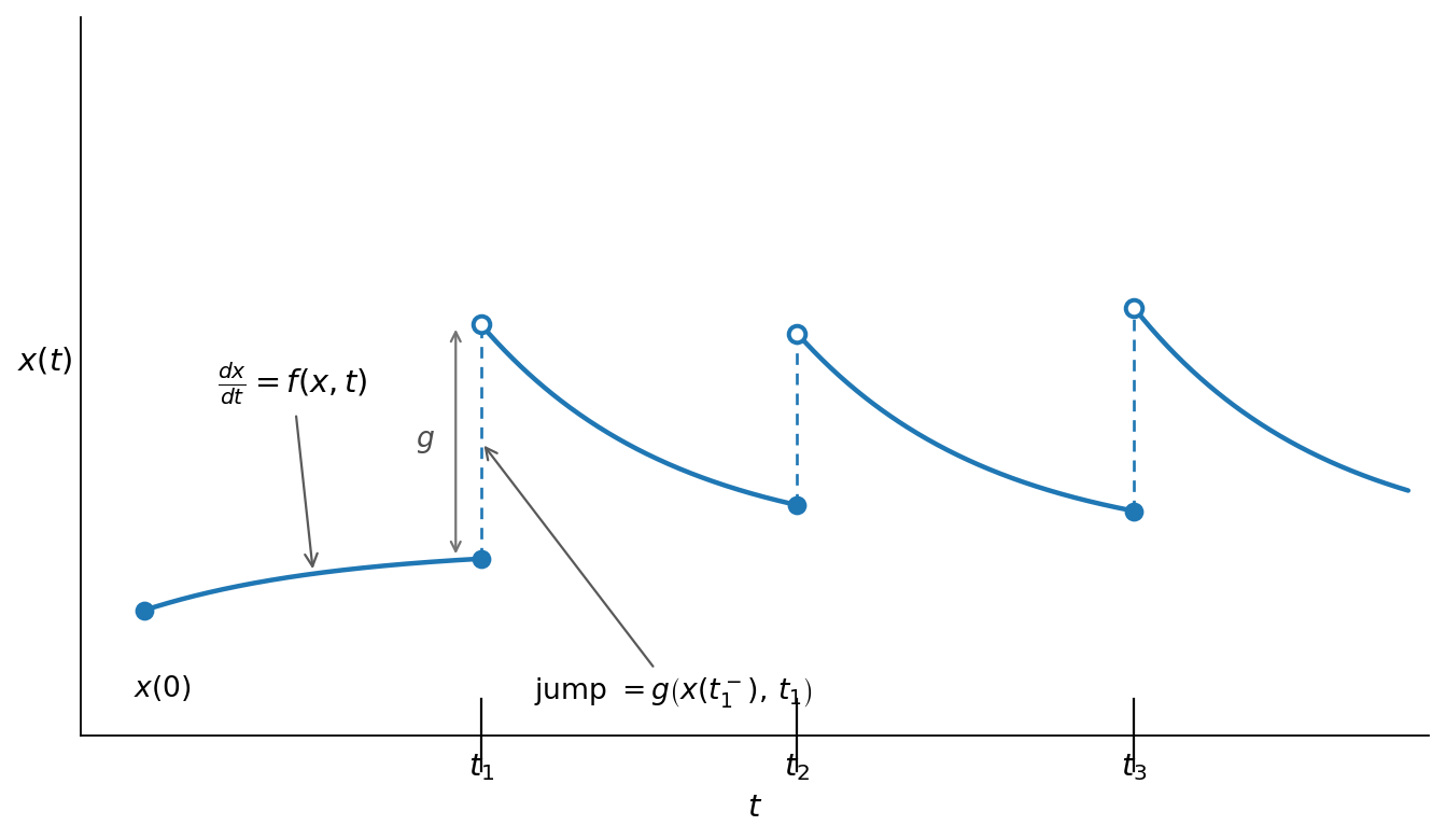
Fig. 3 Figure 1. The solution concept for a Poisson-driven stochastic differential equation. Between the arrival times \(t_i\) the path \(x(t)\) satisfies the ordinary differential equation \(dx/dt = f(x,\, t)\) (the smooth segments). At each arrival time \(t_i\), \(x(t)\) jumps by the amount \(g\bigl(\lim_{t \uparrow t_i} x(t),\, t_i\bigr)\), evaluated at the pre-jump left limit as Definition 9 requires (the dashed vertical segments). The solution is continuous from the left: at \(t_i\) the value \(x(t_i)\) equals the left limit (filled dot), while the post-jump value is the right limit (open dot).

As a first example, consider the stochastic differential equation

\[ dx(t) = xdt + xdN \]

with \(x(0) = 1\).

Using the definition, we find that for \(0 \leq t \leq t_1\),

\[ x(t) = e^{t}. \]

We also find that

\[\begin{split} \begin{aligned} \lim_{t \downarrow t_1}\ x(t) &= \lim_{t \uparrow t_1}\ x(t) + g\ \bigl(\lim_{t \uparrow t_1}\ x(t)\bigr) \\ &= e^{t_1} + e^{t_1} = 2e^{t_1}. \end{aligned} \end{split}\]

Therefore

\[\begin{split} \begin{aligned} x(t) &= 2e^{t_1} \cdot e^{(t - t_1)}\ \text{ for }\ t_1 < t \leq t_2 \\ &= 2e^t\ \text{ for } t_1 < t \leq t_2. \end{aligned} \end{split}\]

Continuing, we find that

\[ x(t) = 4e^t\ \text{ for }\ t_2 < t \leq t_3, \]

and so on.

As our second example, we characterize the solution of the stochastic differential equation

\[ dx(t) = -2x(t)dN(t), \]

subject to \(x(0) = 1\). Applying the definition of a solution, we find that

\[\begin{split} \begin{aligned} x(t) &= 1 \qquad \text{for }\ 0 < t \leq t_1 \\ &-1 \qquad \text{for }\ t_1 < t \leq t_2 \\ &\ \vdots \end{aligned} \end{split}\]

or

\[\begin{split} x(t) = \begin{cases} 1 &\qquad \text{for }\ t_{i-1} < t \leq t_i \qquad i =\ \text{ odd, }\ \ i > 0 \\ -1 &\qquad \text{for }\ t_i < t \leq t_{i+1} \end{cases} \end{split}\]

This stochastic process, which switches between \(+1\) and \(-1\) at the random arrival times \(t_i\), is called a random telegraph wave.

It is also possible to characterize a random telegraph in terms of a pair of functions

\[\begin{split} \begin{aligned} p_1(t) &= \text{Prob}\, \bigl\{x(t) = 1\bigr\} \\ p_{-1}(t) &= \text{Prob}\, \bigl\{x(t) = -1\bigr\} \end{aligned} \end{split}\]

The probabilities \(p_1(t)\), \(p_{-1}(t)\) evolve according to

\[\begin{split} \frac{d}{dt}\ \begin{pmatrix} p_1(t) \\ p_{-1}(t) \end{pmatrix} = \begin{pmatrix} -\lambda & \lambda \\ \lambda & -\lambda \end{pmatrix}\ \begin{pmatrix} p_1(t) \\ p_{-1}(t) \end{pmatrix}, \end{split}\]

subject to \(p_1(0) + p_{-1}(0) = 1\), where \(\lambda\) is the rate of the Poisson counter \(N(t)\).

We can also give a representation of the sample paths of a random telegraph wave as

\[ x(t) = u(t) + 2 \sum_{j=1}^{\infty}\, (-1)^j\, u(t-t_j) \]

where \(\{t_j\}\) are the random arrival times of a Poisson counter with rate \(\lambda > 0\). The generalized derivative of the process can be represented

\[ dx(t)/dt = \delta(t) + 2 \sum_{j=1}^{\infty}\, (-1)^j\, \delta(t-t_j). \]

We now describe three useful rules for manipulating stochastic differential equations that are driven by Poisson counting processes. In 7. Stochastic Differential Equations Driven by a Wiener Process the Wiener-driven analogues of these same three rules, Itô’s rule among them, are obtained as the \(\lambda \to \infty\) limit of the ones developed here. We consider an \(n \times 1\) vector stochastic process \(x(t)\) that is governed by

\[ dx(t) = f\bigl(x(t),\, t\bigr) dt + \sum_{i=1}^{m}\, g_i\bigl(x(t),\,t\bigr) dN_i(t) \]

where \(f\): \(R^n \to R^n,\ g_i\): \(R^n \to R^n\), and \(N_1(t),\ \ldots,\ N_m(t)\) are statistically independent Poisson counting processes with rates \(\lambda_1,\ \ldots,\ \lambda_m\). We consider a vector function \(\Psi(x)\): \(R^n \to R^k\).

Then it follows immediately from Definition 9 that \(\Psi(x)\) satisfies the stochastic differential equation

(20)\[\begin{split} \begin{aligned} d\Psi(x) &= \left\langle \frac{\partial \Psi}{\partial x},\ f(x,\,t)\right\rangle\ dt \\[4pt] &+ \sum_{i=1}^{m}\ \bigl(\Psi\bigl(x + g_i(x,\, t)\bigr) - \Psi(x)\bigr) dN_i(t). \end{aligned} \end{split}\]

Together with Definition 9, equation (20) states that:

(i) in intervals in which there are no arrivals, \(\Psi(x)\) satisfies the ordinary differential equation \(d\Psi(x)/dt = \left\langle \frac{\partial \Psi}{\partial x},\ f(x,\,t)\right\rangle\ dt\); (ii) at arrival times \(t_j\) of any of the \(N_i(t)\) processes

\[\begin{split} \begin{aligned} \lim_{t\downarrow t_j}\ \Psi\bigl(x(t)\bigr) &= \lim_{t \uparrow t_j}\ \Psi\bigl(x(t)\bigr) \\ &+ \Psi\, \bigl[\lim_{t\uparrow t_j}\ \bigl(x(t) + g_i\bigl(x(t),\, t\bigr)\bigr)\bigr] - \Psi\, \bigl(\lim_{t \uparrow t_j}\ x(t)\bigr). \\ &= \Psi\, \bigl[\lim_{t \uparrow t_j}\ \bigl(x(t) + g_i\bigl(x(t),\, t\bigr)\bigr)\bigr]. \end{aligned} \end{split}\]

(iii) \(\Psi(x(t))\) is continuous from the left.

Notice that since \(\lim_{t\downarrow t_j}\ x(t) = \lim_{t \uparrow t_j}\ (x(t) + g_i(x(t),\, t)))\), the rule (20) and its implication delivers the property that the solution \(\Psi(x)\) is the desired function \(\Psi(x)\) at all points, including the arrival times \(t_j\), which are the discontinuities of \(x(t)\).

As an example of the use of this rule, we desire to find a differential equation for

\[ y = x^2 \]

where \(x(t)\) obeys

\[ dx = -xdt + dN_1 - dN_2 \]

We set \(\Psi(x) = x^2\), and find

\[ dx^2 = \left\langle 2x,\, -x\right\rangle\, dt + \bigl((x+1)^2 - x^2\bigr)\, dN_1 + \bigl((x-1)^2 - x^2\bigr)\,dN_2 \]

or

\[ dx^2 = -2x^2\, dt + (2x+1) dN_1 + (-2x+1) dN_2. \]

As a second example, take the differential equation that generates the random telegraph wave,

\[ dx = -2xdN,\ \text{ with }\ x(0) = 1. \]

We want to find a stochastic differential equation for \(y = x^2\),

\[ dx^2 = \bigl((x - 2x)^2 - x^2\bigr)dN \]

or

\[ dx^2 = 0 \]

With the initial condition \(x(0)^2 = 1\), this implies that \(x^2(t) = 1\) for all \(t \geq 0\).

We now describe a second rule that is useful for computing expectations. We consider the differential equation

\[ dx(t) = f(x,\, t)dt + \sum_{i=1}^{m}\, g_i\bigl(x(t),\, t\bigr) dN_i(t) \]

where the \(N_i(t)\) are \(m\) independent Poisson counters with rates \(\lambda_i\). We seek to evaluate

(21)\[\begin{split} \begin{aligned} E\, \bigl(x(t + \Delta) - x(t)\bigr) &= E\, \int_t^{t + \Delta}\ f\bigl(x(s),\, s\bigr)ds \\ &+ \sum_{i=1}^{m}\ E\ \int_t^{t+\Delta}\ g_i\, \bigl(x(s),\, s\bigr)dN_i(s) \end{aligned} \end{split}\]

We express the second integral using

(22)\[\begin{split} \begin{aligned} E\, \int_t^{t + \Delta} &\ g_i\, \bigl(x(s),\, s\bigr) dN_i(s) = E\, \int_t^{t + \Delta}\ g_i\, \bigl(x(s),\, s\bigr)\ (dN_i - \lambda_i\, ds) \\ &+ E\, \int_t^{t + \Delta}\ \lambda_i\, g_i\, \bigl(x(s),\, s\bigr)ds. \end{aligned} \end{split}\]

We now use the following two properties of the Poisson counter: (a) \(E(N_i(t) - \lambda_i t) = 0\), (b) the probability that \(N_i(t)\) jumps in \([t,\, t + \Delta]\) is independent of \(x(t)\).

These imply that \(E \int_t^{t + \Delta}\, g_i\, (x(s),\, s)\ (dN_i - \lambda_i\, ds) = 0\).

Using this result in (21) and (22), dividing by \(\Delta\), and taking the limit as \(\Delta \to 0\) gives

(23)\[ \frac{d}{dt}\ Ex(t) = Ef\,\bigl(x(t),\, t\bigr) + \sum_{i=1}^{m}\, E g_i\, \bigl(x(t),\, t\bigr)\, \lambda_i. \]

As an example of the use of (23), we reconsider the stochastic differential equation

\[ dx = -x(t) dt + dN_1 - dN_2 \]

which implied

\[ dx^2 = -2x^2 dt + (2x+1) dN_1 + (-2x+1)dN_2 \]

where \(N_1\) and \(N_2\) are independent Poisson counters with rates \(\lambda_1\) and \(\lambda_2\). Applying rule (23), we find that

\[\begin{split} \begin{aligned} \frac{d}{dt}\ Ex(t) &= -Ex(t) + \lambda_1 - \lambda_2. \\[4pt] \frac{d}{dt}\ Ex(t)^2 &= -2Ex^2 + E(2x + 1)\, \lambda_1 + E\, (-2x + 1)\, \lambda_2. \end{aligned} \end{split}\]

We now derive a third rule, which can be used to calculate the autocorrelation function of the \(x(t)\) process. We again consider the stochastic differential equation

\[ dx(t) = f\, \bigl(x(t),\, t\bigr) dt + \sum_{i=1}^{m}\, g_i\, \bigl(x(t),\, t\bigr) dN_i(t). \]

We express the solution as

\[ x(\tau) = x(0) + \int_0^\tau\, f\bigl(x(s),\, s\bigr)ds + \sum_i \int_0^\tau\, g_i\, \bigl(x(s),\, s\bigr) dN_i(s). \]

For \(t < \tau\), we have

\[\begin{split} \begin{aligned} x(t) x(\tau) &= x(0) x(t) + \int_0^\tau \, x(t)\, f\bigl(x(s),\, s\bigr) ds \\ &+ \sum_i\, \int_0^\tau\, x(t) g\bigl(x(s),\, s\bigr)dN_i(s). \end{aligned} \end{split}\]

Taking expectations of both sides gives

\[\begin{split} \begin{aligned} Ex(t) x(\tau) &= Ex(0) x(t) + E \int_0^\tau \, x(t) f\bigl(x(s),\, s\bigr) ds \\ &+ \sum_i \, E \int_0^\tau\, x(t) g\bigl(x(s),\, s\bigr) dN_i(s) \end{aligned} \end{split}\]

We also express this equation as

\[ dEx(t) x(\tau) = Ex(t) f\bigl(x(\tau),\, \tau\bigr) d\tau + E \sum_i x(t) g_i\, \bigl(x(\tau),\, \tau\bigr) dN_i(\tau) \]

which implies, via our rule (23), that

\[\begin{split} \begin{aligned} & \frac{d}{d\tau}\ Ex(t) x(\tau) = Ex(t) f\bigl(x(\tau),\, \tau\bigr) + \sum_i Ex(t) g_i\, \bigl(x(\tau),\, \tau\bigr) \lambda_i. \\ &\tau > t. \end{aligned} \end{split}\]

Equivalently, we can express this rule as

(24)\[\begin{split} \begin{aligned} \frac{d}{d\tau}\ Ex(t) x(t + \tau) &= Ex(t) f\bigl(x(t + \tau),\, t+ \tau\bigr) \\ &+ \sum_i\, Ex(t) g_i\, \bigl(x(t + \tau),\, t+ \tau\bigr)\, \lambda_i. \\ &\ \tau > 0. \end{aligned} \end{split}\]

As an example, consider the random telegraph wave, which is determined by the solution to the stochastic differential equation

\[ dx(t) = -2xdN,\ x(0) = 1. \]

We have

\[ dx(t) x(t + \tau) = -2x(t) x(t + \tau)dN(t + \tau). \]

This implies that

\[ \frac{d}{d\tau}\ Ex(t) x(t + \tau) = -2\lambda\, Ex(t) x(t + \tau),\ \tau > 0 \]

or

\[ \frac{d}{d\tau}\ R\, (t,\, t+\tau) = -2\lambda\, R(t,\, t+\tau),\ \tau > 0 \]

The solution of this differential equation in \(\tau\) is

\[ R(t,\, t + \tau) = e^{-2\lambda\tau}\, R(t,\, t),\ \tau > 0. \]

If we start the random telegraph wave with random initial condition \(\text{Prob }\, \{x(0) = 1\} = \text{ Prob }\, \{x(0) = -1\} = 1/2\), we find that

\[ \frac{d}{dt}\ Ex(t) = -2\lambda\, Ex(t), \]

which implies that

\[ Ex(t) = e^{-2\lambda t}\, E\bigl(x(0)\bigr) \]

so that

\[ Ex(t) = 0 \, \text{ for all } \, t. \]

In this case, the random telegraph wave is a stationary stochastic process, and has autocorrelation function given by

\[ R(\tau) = e^{-2\lambda |\tau|}. \]

Note that the random telegraph wave is mean square continuous, but not mean square differentiable.

As a second example, consider the stochastic differential equation

\[ dx(t) = -ax(t)dt + (dN_1 - dN_2),\ a > 0 \]

where \(N_1\) and \(N_2\) are two Poisson counters with identical rates \(\lambda\). Applying (24), we find that

\[ \frac{d}{d\tau}\ Ex(t) x(t+\tau) = -aEx(t) x(t+\tau),\ \tau > 0 \]

which implies that

\[ R(t,\, t + \tau) = e^{-a\tau} R(t,\,t). \]

A useful example is the stochastic process \(x(t)\) governed by the stochastic differential equation

\[ dx = \frac{1}{\sqrt\lambda}\ (dN_1 - dN_2) \]

with \(x(0) = 0\), and where \(N_1\) and \(N_2\) are independent Poisson counting processes each with rate \(\lambda/2\). Applying formulas (23), we find that

\[ \frac{d}{dt}\ Ex(t) = \frac{1}{\sqrt \lambda}\ (\lambda/2 - \lambda/2) = 0 \]

which, together with \(x(0) = 0\), implies that

\[ Ex(t) = 0\ \text{ for all }\ t \geq 0. \]

We use formula (20) to derive a differential equation for \(x^2\), namely

\[\begin{split} \begin{aligned} dx(t)^2 &= \Bigl[(x + 1/\sqrt\lambda\,)^2 - x^2\Bigr]\, dN_1 \\ &+ \Bigl[(x - 1/\sqrt\lambda\,)^2 - x^2\Bigr]\, dN_2 \end{aligned} \end{split}\]

or

\[ dx(t)^2 = \bigl[2x/\sqrt\lambda + 1/\lambda\bigr]\, dN_1 + \bigl[-2x/\sqrt\lambda + 1/\lambda\bigr]\, dN_2 \]

Applying formula (23) to the above equation, we find that

\[ \frac{d}{dt}\, Ex(t)^2 = \bigl[2\, Ex/\sqrt\lambda + 1/\lambda\bigr]\, \lambda/2 + \bigl[-2Ex/\sqrt\lambda + 1/\lambda\bigr]\,\lambda/2 = 1. \]

Since \(x(0) = 0\) implies that \(Ex(0)^2 = 0\), the above ordinary differential equation for \(Ex(t)^2\) has the solution

\[ Ex(t)^2 = t. \]

Finally, applying formula (24), we have that for \(\tau > 0\)

\[ \frac{d}{d\tau}\ Ex(t) x(t +\tau) = Ex(t)\ \frac{1}{\sqrt \lambda}\ (\lambda/2 - \lambda/2) = 0. \]

Therefore, we have that

\[ R(t,\, t + \tau) = t\ \text{ for }\ \tau > 0. \]

In summary, the process governed by the differential equation

\[ dx = \ \frac{1}{\sqrt \lambda}\ (dN_1 - dN_2) \]

where \(N_1\) and \(N_2\) are independent Poisson counters with rate \(\lambda/2\), is an example of a random walk. It has mean zero and autocorrelation function

\[ R(t,\, t + \tau) = \min\ (t, \, t + \tau). \]

The process is mean square continuous, but not mean square differentiable. Its derivative exists only in the sense of a “generalized stochastic process.” This random walk, taken to the limit \(\lambda \to \infty\), is precisely the construction from which the Wiener process is obtained in 6. The Wiener Process.

As our next example, we give alternative representations of the “generalized Poisson process.” Let \(a(t)\) be a continuum of independent, identically distributed normal random variables each with mean zero and variance \(\sigma_a^2\). A generalized Poisson process \(y(t)\) can then be represented as

\[ y(t) = \sum_{i=1}^{\infty}\ a(\tau_i)\, u(t - \tau_i) \]

or

(25)\[ \frac{dy(t)}{dt}\ = \sum_{i=1}^{\infty}\ a(\tau_i)\, \delta(t - \tau_i) \]

where \(\tau_i\) is the \(i^{th}\) arrival time of a Poisson counter with rate \(\lambda\). An alternative representation in terms of an Ito stochastic differential equation is

\[ dy(t) = a(t)dN(t) \]

where \(N(t)\) is a Poisson counting process with rate \(\lambda\) and where the normal random variate \(a(t)\) enters as \(g(x(t),\, t)\) in formula (19). Applying rule (20) to derive a differential equation for \(y(t)^2\), we obtain

\[ dy(t)^2 = \bigl[a(t)^2 + 2a(t) y(t)\bigr]\, dN(t). \]

Since \(a(t)\) is independent of \(y(t)\), applying rule (23), we find

\[ \frac{d}{dt}\ Ey(t)^2 = \sigma_a^2 \lambda. \]

so that

\[ Ey(t)^2 = (\sigma_a^2 \lambda) t. \]

We also have

\[ \frac{d}{dt}\ Ey(t) = \lambda Ea(t) = 0. \]

Finally, for \(\tau > 0\), we have from rule (24) that

\[ dEy(t) y(t + \tau) = Ey(t) a(t + \tau) \cdot \lambda = 0. \]

Therefore, for \(\tau > 0\),

\[ Ey(t) y(t + \tau) = Ey(t)^2 = \sigma_a^2 \lambda t. \]

Thus, the generalized Poisson process is a random walk. At the random arrival times \(\tau_i\), the process \(y(t)\) takes a jump of random size \(a(\tau_i)\). Since the normal distribution that governs \(a(\tau_i)\) is symmetric about zero, the process is as likely to jump upward as it is to jump downward. This is why the process has no “drift,” i.e., it has zero mean for all \(t\). The process is mean square continuous, but not mean square differentiable. The derivative \(dy(t)/dt\) given by (25) exists in the sense of a generalized stochastic process. This derivative is an example of a white noise, its autocorrelation function being a delta function \(\sigma_a^2 \lambda \delta(\tau)\). In our work below, such a white noise is a valid input into a linear system. For example, if we define

(26)\[ w(t) = \frac{dy(t)}{dt} = \sum_{i=1}^{\infty}\ a(\tau_i)\, \delta(t - \tau_i) \]

we might be interested in the process,

(27)\[ z(t) = \int_0^\infty h(\tau)\, w(t - \tau) d\tau \]

where \(h(\tau)\) is a continuous function in \(L_2\, [0,\, \infty]\). By substituting (26) into (27) and exchanging orders of integration and summation, we find that

\[ z(t) = \sum_{i=1}^{\infty}\ a(\tau_i)\, h(t - \tau_i). \]

Later, the process \(z(t)\) will be shown to be a covariance stationary one for which the first and second moments are readily computed.

Exercises

import numpy as np
import matplotlib.pyplot as plt

Exercise 3

The random telegraph wave switches between \(+1\) and \(-1\) at the arrival times of a Poisson counter of rate \(\lambda\). Equivalently, if \(N(t)\) is the counter and \(x(0)\) is \(\pm 1\) with equal probability, then

\[ x(t) = x(0)\, (-1)^{N(t)}. \]

When the initial sign is equally likely to be \(+1\) or \(-1\), the text shows the process is stationary with mean zero and autocorrelation

\[ R(\tau) = e^{-2\lambda|\tau|}. \]

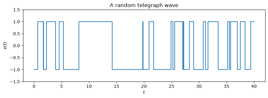
(a) Simulate and plot one sample path with \(\lambda = 1\).

(b) Estimate the autocovariance \(R(\tau)\) by averaging \(x(t)\,x(t+\tau)\) over an ensemble of simulated paths, and compare it with \(e^{-2\lambda\tau}\).

Solution to Exercise 3

The sign of \(x(t)\) flips each time the Poisson counter advances, so on a time grid we only need the number of arrivals up to each grid point. We obtain that count by searching the sorted arrival times.

rng = np.random.default_rng(0)

def telegraph_path(lam, grid, rng):
    """A random telegraph wave sampled on `grid`, with random initial sign."""
    T = grid[-1]
    times, t = [], 0.0
    while True:
        t += rng.exponential(1.0 / lam)
        if t > T:
            break
        times.append(t)
    n_arrivals = np.searchsorted(np.array(times), grid, side='right')
    x0 = rng.choice([-1.0, 1.0])
    return x0 * (-1.0) ** n_arrivals

lam = 1.0
dt = 0.02
grid = np.arange(0.0, 40.0 + dt, dt)

# (a) one sample path
fig, ax = plt.subplots(figsize=(10, 3))
ax.step(grid, telegraph_path(lam, grid, rng), where='post')
ax.set_ylim(-1.5, 1.5); ax.set_xlabel('$t$'); ax.set_ylabel('$x(t)$')
ax.set_title('A random telegraph wave')
plt.show()

# (b) estimate the autocovariance over an ensemble of paths
n_paths = 1500
L = len(grid)
X = np.empty((n_paths, L))
for i in range(n_paths):
    X[i] = telegraph_path(lam, grid, rng)

max_lag = int(2.0 / dt)
acf = np.array([np.mean(X[:, :L - k] * X[:, k:]) for k in range(max_lag)])
taus = np.arange(max_lag) * dt

fig, ax = plt.subplots(figsize=(8, 4))
ax.plot(taus, acf, 'o', ms=3, label=r'simulated $R(\tau)$')
ax.plot(taus, np.exp(-2 * lam * taus), 'r-', lw=2, label=r'$e^{-2\lambda\tau}$')
ax.set_xlabel(r'$\tau$'); ax.set_ylabel(r'$R(\tau)$')
ax.legend()
plt.show()

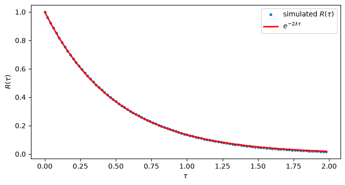
The simulated autocovariance falls on the exponential \(e^{-2\lambda\tau}\), confirming the analytical result. Note that \(R(\tau)\) has a kink at \(\tau = 0\): the telegraph wave is mean square continuous but not mean square differentiable.