7. Stochastic Differential Equations Driven by a Wiener Process#
We wish to consider a class of stochastic differential equations driven by a Wiener process,
We shall derive rules for manipulating such equations by regarding (33) as the limit as \(\lambda \to \infty\) of
where \(N_1\) and \(N_2\) are two independent Poisson counters with identical rates \(\lambda/2\).
The first rule we seek is the counterpart of rule (20). Where \(\Psi(x)\) is a function of \(x\), \(\Psi(x)\) obeys the differential equation
Note
Throughout this chapter, \(\langle u,\, v\rangle\) denotes the Euclidean inner product of two vectors \(u\) and \(v\) in \(\mathbb{R}^n\),
Here \(x\) is a vector-valued state, \(\Psi(x)\) is a scalar-valued function, \(\dfrac{\partial\Psi}{\partial x}\) is its gradient, a column vector with entries \(\partial\Psi/\partial x_i\), and \(\dfrac{\partial^2\Psi}{\partial x^2}\) is its Hessian, the matrix of second partials \(\partial^2\Psi/\partial x_i\,\partial x_j\). With this reading,
\(\left\langle \dfrac{\partial\Psi}{\partial x}\, ,\ f\right\rangle = \sum_i \dfrac{\partial\Psi}{\partial x_i}\, f_i\) pairs the gradient with the drift vector \(f\); and
\(\left\langle \dfrac{\partial^2\Psi}{\partial x^2}\, g,\ g\right\rangle = g^\top \dfrac{\partial^2\Psi}{\partial x^2}\, g = \sum_{i,\,j} \dfrac{\partial^2\Psi}{\partial x_i\,\partial x_j}\, g_i\, g_j\) is the quadratic form in the diffusion vector \(g\). The Hessian acts on \(g\), and then we take the inner product with \(g\) again.
When \(x\) is scalar, every inner product collapses to ordinary multiplication: \(\langle \Psi', f\rangle = \Psi' f\) and \(\langle \Psi'' g,\, g\rangle = \Psi'' g^2\). The scalar example at the end of this chapter uses that form.
To generate this rule, we use (34) for \(\lambda > 0\) and using rule (20) to obtain
Obtain for \(\Psi(x \pm\, \frac{1}{\sqrt\lambda}\ g(x,\, t))\) its Taylor series expansion about \(x\),
where \(0\, (\frac{1}{\lambda^{3/2}}) \to 0\) as \(\lambda \to \infty\). Substituting the Taylor expansions in (35), we obtain
Now consider the process \(z(t)\) governed by
Applying our rules, we find that
so that
We also find that
so that as \(\lambda \to \infty\)
Therefore
It follows that
which implies that as \(\lambda \to \infty\),
with probability 1.
Thus returning to (36) and taking limits as \(\lambda \to \infty\), we obtain
This is known as Ito’s rule for the stochastic differential equation
Later chapters use Itô’s rule sparingly. The linear theory of 11. Linear Stochastic Differential Equations and 12. Linear Least Squares Prediction integrates white noise against a deterministic kernel \(p(\tau)\). For such an integrand the second-order term above vanishes, and the Itô integral, the Stratonovich integral, and the ordinary mean square integral coincide. A note in 11. Linear Stochastic Differential Equations records this.
The correction does work in one place, the derivation of the Riccati equation of the Kalman–Bucy filter in 15. State-Space Models, the Kalman Filter, and Spectral Factorization. Applying the rule to the quadratic function \(\Psi(e) = e\,e^\top\) of the estimation error, the second-order term supplies the noise-intensity terms \(BB^\top + KRK^\top\) that the Riccati equation balances against \(\Sigma C^\top R^{-1} C\,\Sigma\). Chapters 5 through 7 otherwise serve to construct the white noise that the linear theory takes as given, from Poisson and Wiener cases by one limiting argument.
Our second rule is
This rule can be derived by the same limiting process. For \(\lambda > 0\), we have
which implies that
the factor \(\lambda/2\) being the common rate of each of the two counters.
Now take Taylor series expansions of \(\Psi\, (x \pm\, \frac{1}{\sqrt\lambda}\ g(x,\, t))\) about \(x\) to get
The first-order terms cancel between the two counters; the two second-order terms are identical, so together they contribute \((1/\lambda)\langle \Psi_{xx} g,\, g\rangle\), which the rate \(\lambda/2\) converts into \(\tfrac12 \langle \Psi_{xx} g,\, g\rangle\).
Taking the limit as \(\lambda \to \infty\) gives the desired result (37).
The next result that we desire is for \(\tau > 0\),
To obtain this, we take limits as \(\lambda \to \infty\) in the formula
As an example of the use of these formulas, we take the linear stochastic differential equation, the Ornstein–Uhlenbeck process, the simplest member of the constant-coefficient class that 11. Linear Stochastic Differential Equations studies systematically,
Applying our formulas, we find that
Exercises#
The linear stochastic differential equation
is the Ornstein–Uhlenbeck process. The exercises below simulate it and check the moment formulas just derived. We simulate using the Euler–Maruyama scheme: on a grid of spacing \(dt\),
which simply discretizes \(dx = -a x\, dt + b\, dW\) with \(dW = \sqrt{dt}\,\varepsilon\).
import numpy as np
import matplotlib.pyplot as plt

def ou_paths(a, b, T, dt, n, rng, x0=0.0):
    """Simulate n Ornstein-Uhlenbeck paths on [0, T] via Euler-Maruyama."""
    steps = int(T / dt)
    X = np.empty((n, steps + 1))
    X[:, 0] = x0
    s = b * np.sqrt(dt)
    for k in range(steps):
        X[:, k + 1] = X[:, k] - a * X[:, k] * dt + s * rng.normal(size=n)
    return X
Exercise 6
Take \(a = 1\), \(b = 0.7\), and start all paths at \(x(0) = 0\).
The text’s equations integrate (with \(x(0)=0\)) to the transient variance
which approaches the stationary variance \(b^2/(2a)\) as \(t \to \infty\).
(a) Simulate an ensemble of paths and plot a handful of them together with the theoretical \(\pm\) one-standard-deviation band \(\pm\sqrt{E\,x(t)^2}\).
(b) Check that the variance across paths at the final time matches the stationary value \(b^2/(2a)\).
Solution to Exercise 6
rng = np.random.default_rng(3)
a, b = 1.0, 0.7
dt, T, n = 0.02, 20.0, 8000

X = ou_paths(a, b, T, dt, n, rng)
t = np.arange(X.shape[1]) * dt

# (a) sample paths and theoretical std band
sd = np.sqrt((b**2 / (2 * a)) * (1 - np.exp(-2 * a * t)))
fig, ax = plt.subplots(figsize=(10, 4))
for i in range(5):
    ax.plot(t, X[i], lw=0.8)
ax.plot(t, sd, 'k--', lw=2, label=r'theoretical $\pm\sqrt{E\,x(t)^2}$')
ax.plot(t, -sd, 'k--', lw=2)
ax.set_xlabel('$t$'); ax.set_ylabel('$x(t)$')
ax.set_title('Ornstein–Uhlenbeck paths and the growing variance band')
ax.legend()
plt.show()

# (b) stationary variance
print(f"variance at t={T}: simulated {X[:, -1].var():.4f},  theory b^2/2a = {b**2 / (2 * a):.4f}")
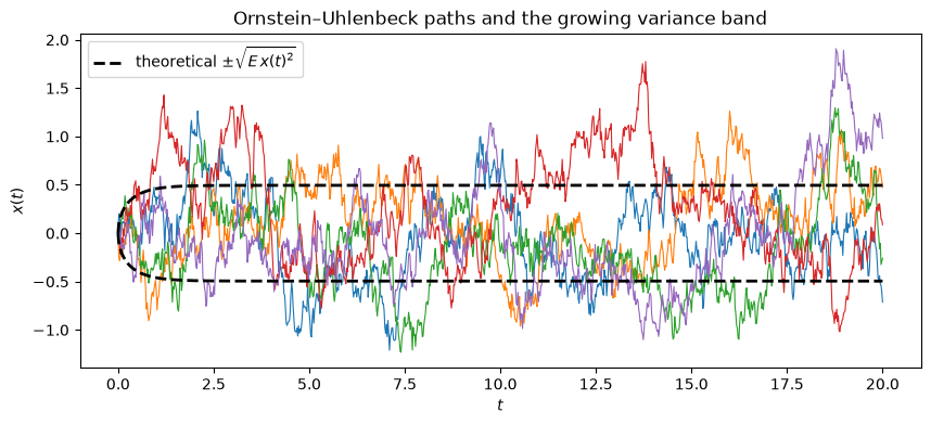
variance at t=20.0: simulated 0.2433, theory b^2/2a = 0.2450
The paths fan out from \(0\) and settle into a stationary band whose width is the mean-reverting balance between the diffusion \(b\,dW\) pushing the process out and the drift \(-a x\,dt\) pulling it back.
Exercise 7
In the stationary regime the text shows the autocovariance decays exponentially,
Continuing the simulation from Exercise 6, discard an initial burn-in so the process is (approximately) stationary, then estimate the normalized autocovariance \(R(\tau)/R(0)\) by averaging \(x(t)\,x(t+\tau)\) over both time and paths. Compare it with \(e^{-a\tau}\).
Solution to Exercise 7
burn = int(10.0 / dt)            # drop the first 10 time units
Xs = X[:, burn:]
Xs = Xs - Xs.mean()
R0 = np.mean(Xs * Xs)

lags = np.arange(0, int(4.0 / dt))
acf = np.array([np.mean(Xs[:, :Xs.shape[1] - k] * Xs[:, k:]) for k in lags]) / R0
taus = lags * dt

fig, ax = plt.subplots(figsize=(8, 4))
ax.plot(taus, acf, 'o', ms=3, label=r'simulated $R(\tau)/R(0)$')
ax.plot(taus, np.exp(-a * taus), 'r-', lw=2, label=r'$e^{-a\tau}$')
ax.set_xlabel(r'$\tau$'); ax.set_ylabel(r'$R(\tau)/R(0)$')
ax.legend()
plt.show()
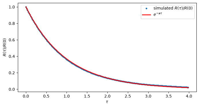
The estimated autocovariance tracks \(e^{-a\tau}\). Note that \(R(\tau) = R(0)e^{-a|\tau|}\) has a kink at \(\tau = 0\), like the \(e^{-2\lambda|\tau|}\) of the telegraph wave of Chapter 5, and for the same reason. The kink means that \(R'(0^+) = -aR(0)\) while \(R'(0^-) = +aR(0)\), so \(R''(0)\) does not exist; by Theorem 4 of 2. Mean Square Continuity and Differentiability of a Stochastic Process the Ornstein–Uhlenbeck process is therefore, like the telegraph wave, mean square continuous but not mean square differentiable. In the language of 11. Linear Stochastic Differential Equations this is the case \(n = 1\), \(m = 0\), giving \(n - 1 - m = 0\) derivatives; by 13. Locally Unpredictable Stochastic Processes such a process is locally unpredictable. The two processes differ in their sample paths, since the diffusion is continuous and the telegraph wave jumps. Their second moments are alike in this respect.