8. Spectral Densities#
(a) General Results#
Let \(x(t)\) be a covariance stationary stochastic process with covariogram
where \(R\) is a positive semidefinite function. Covariogram names the same function that 1. Covariance Stationary Stochastic Processes calls the autocorrelation function \(R(\tau)\) and, for a zero mean process, the autocovariance function \(C(\tau)\). All three names appear in this book, and the note in that chapter explains why. The power spectrum or the spectral density of \(x\) is defined as
Equation (38) defines \(S(\omega)\) as the Fourier transform of \(R(\tau)\). Given \(S(\omega)\), \(R(t)\) can be recovered from the inverse Fourier transform
From the fact that \(R(\tau)\) is a positive semidefinite function, which implies that \(R(\tau) = R(-\tau)\), definition (38) and the inverse relation (39) imply that \(S(\omega)\) has the following properties
(i) \(S(\omega) = S(-\omega)\). (from definition (38))
(ii) \(S(\omega) \geq 0\). (from definition (38) and positive semidefiniteness of \(R(t)\))
(iii) \(\frac{1}{2\pi} \int_{-\infty}^{\infty} S(\omega)\, d\omega = R(0)\quad\) ((39) evaluated at \(\tau = 0\))
Property (iii) asserts that the spectral density achieves a decomposition of the variance \(R(0)\) by frequency. We shall shortly see that this decomposition of variance is actually into components that are orthogonal across different frequencies.
For the purposes of using (38) and (39), it is fortunate that tables of Fourier transform pairs have been prepared. Table 1 is a small table. The reader can verify the entries in the table by using (38) or (39).
Fourier transforms have a number of useful operational properties. In particular, let \(F(\omega) \leftrightarrow f(t)\) mean that \(F(\omega)\) is the Fourier transform of the “time signal” \(f(t)\), i.e.,
Then a number of simple operations of \(F(\omega)\) or \(f(t)\) can be used to generate other Fourier transform pairs. Some of these are recorded in table 2.
Property (8) of table 2 can be used to find the spectral density of mean square derivatives of a given process \(x(t)\). We saw above that if \(x_t\) is a covariance stationary stochastic process with autocovariogram \(R(\tau)\), then the autocovariogram of \(\frac{d^n}{dt^n}\ x(t)\) is \((-1)^n\ \frac{d^{2n} R(\tau)}{d\tau^{2n}}\). It follows from property 8 of table 2 that the Fourier transform of \((-1)^n \ \frac{d^{2n}R(\tau)}{d\tau^{2n}}\) is \(\omega^{2n}F(\omega)\), where \(F(\omega)\) is the Fourier transform of \(R(\tau)\).
The preceding property can be viewed as a limiting case of a more general property. Let \(x(t)\) be a covariance stationary process with covariogram \(R(\tau)\). Define \(y(t)\) as
where \(h(\tau) \in L_2\, [-\infty,\, \infty]\). Then calculating \(Ey(t)y(t-s)\) gives
Applying property 6 of table 2, the convolution property, twice to (40), together with property 12 (reversal) to handle the \(h(-s)\) factor, gives
where \(h(\omega) = \int_{-\infty}^{\infty} h (\tau) e^{-i \omega \tau}\, d\tau\) is the Fourier transform of \(h(t)\).
The sense in which our preceding result is a special case of (40) is as follows. The generalized derivative of \(\delta (t),\ \delta' (t)\), is a generalized function defined by
where \(g' (t)\) is a test function that is differentiable at \(t = 0\). More generally, the \(n^{th}\) generalized derivative of \(\delta (t)\) is defined by
where \(g(t)\) is a test function that is \(n\) times differentiable at \(t\). See Papoulis for definitions of \(\delta (t)\) and its generalized derivatives. Both \(\delta (t)\) and \(\delta^{(n)}\, (t)\) can be defined in terms of particular limit points of sequences of functions \(h_n (t) \in L_2 [-\infty, \, \infty]\) for each \(n\), which are used as integrating functions in
The Fourier transform of \(\delta' (t)\) is seen to be, from the definition
More generally, the Fourier transform of \(\delta^{(n)} (t)\) is given by
Using this result in conjunction with (41) with \(h(t) = \delta^{(n)} (t)\) immediately gives that the spectrum of the \(n^{th}\) mean square derivative of a process \(x(t)\) with spectrum \(S(\omega)\) is given by \(\omega^{2n} S(\omega)\).
We record some of these results in table 3.
Tables#
Table 1#
\(f(t)\) |
\(F(\omega)\) |
|---|---|
\(e^{-a\vert t\vert}\) |
\(\frac{2a}{a^2 + \omega^2}\), \(a > 0\) |
\(u(t)\) |
\(\frac{1}{i\omega} + \pi\, \delta(\omega)\) |
\(u(t)t\) |
\(\frac{1}{(i\omega)^2} + i\pi\, \delta'(\omega)\) |
\(\delta (t)\) |
\(1\) |
\(\delta' (t)\) |
\(i\omega\) |
\(\delta^{(n)}\, (t)\) |
\((i\omega)^n\) |
\(\sum_{n=-\infty}^{\infty} \delta (\tau-nT)\) |
\(\omega_0 \sum_{n=-\infty}^{\infty} \delta (\omega-n \omega_0),\ \omega_0 = \frac{2\pi}{T}\) |
\(e^{-at}\, u(t)\) |
\(\frac{1}{a + i\omega}\), \(a > 0\) |
\(\begin{cases} 1 & t \in [0,\,1] \\ 0 & t > 1,\ t < 0 \end{cases}\) |
\(\left(\frac{1 - e^{-i\omega}}{i\omega}\right)\) |
\(\begin{cases} 1 & t \in [0,\,1] \\ -1 & t \in [1,\, 2] \\ 0 & t > 2,\ t < 0 \end{cases}\) |
\(\frac{(1 - e^{-i\omega})^2}{i\omega}\) |
\(\begin{cases} t, & t \in [0,\,1] \\ 2-t, & t \in [1,\,2] \\ 0 & t < 0,\ t > 2 \end{cases}\) |
\(\frac{(1-e^{-i\omega})^2}{(i\omega)^2}\) |
\(\frac{t^{n-1}}{(n-1)!}\, e^{-at}\, u(t)\) |
\(\frac{1}{(a+i\omega)^n}\), \(a > 0\) |
\(e^{i\omega_0t}\) |
\(2\pi \delta (\omega-\omega_0)\) |
\(\cos\ \omega_0 t\) |
\(\pi\, \left[\delta (\omega-\omega_0) + \delta\, (\omega+\omega_0)\right].\) |
Note: \(u(t) = \begin{cases} 1 & t \geq 0 \\ 0 & t < 0 \end{cases}\qquad\) (Heaviside step function)
The entries for \(u(t)\) and \(u(t)t\) are the transforms in the sense of generalized functions; the \(\delta\) terms record that these signals do not decay, and they carry all of the mass at \(\omega = 0\). In every use we make of these entries, the operators \(1/(i\omega)\) and \(1/(i\omega)^2\) act on a noise that has no mass at \(\omega = 0\), so the \(\delta\) terms may be, and are, dropped. Those uses are the operational calculus of 11. Linear Stochastic Differential Equations and 12. Linear Least Squares Prediction and the nonstationary examples of 14. Examples of Nonstationary Processes. Writers who work only with such operators often tabulate \(u(t) \leftrightarrow 1/i\omega\) for that reason.
\(\delta (t) =\) Dirac delta generalized function, defined by \(\int_{-\infty}^{\infty} g(t) \delta(t)\, dt = g(0)\) where \(g(t)\) is a “test function” that is continuous at \(t=0\).
Table 2#
Property:
Property |
Transform pair |
|---|---|
1. Linearity |
\(a_1 f_1 (t) + a_2 f_2(t) \leftrightarrow a_1 F_1(\omega) + a_2 F_2 (\omega)\); \(a_1,\ a_2\) are scalars. |
2. Symmetry |
\(F(t) \leftrightarrow 2\pi f(-\omega)\) |
3. Scaling |
\(f(at) \leftrightarrow \frac{1}{\vert a\vert}\ F\left(\frac{\omega}{a}\right),\ \text{ a scalar}\) |
4. Delay |
\(f(t-t_0) \leftrightarrow e^{-i\omega t_0}\, F(\omega)\) |
5. Modulation |
\(e^{i\omega_0t}\, f(t) \leftrightarrow F(\omega-\omega_0)\) |
6. Convolution |
\(f_1(t) \ast f_2(t) \leftrightarrow F_1(\omega)F_2(\omega)\); where \(f_1(t) \ast f_2(t) \equiv \int_{-\infty}^{\infty} f_1(t-\tau) f_2(\tau)\, d\tau\) |
7. Multiplication |
\(f_1(t) f_2 (t) \leftrightarrow \frac{1}{2\pi} F_1 (\omega) \ast F_2 (\omega)\); where \(F_1(\omega) \ast F_2(\omega) \equiv \int_{-\infty}^{\infty} F_1(\omega-s) F_2(s)\, ds\) |
8. Time differentiation |
\(\frac{d^n}{dt^n}\, f(t) \leftrightarrow (i\omega)^n\ F(\omega)\) |
9. Time integration |
\(\int_{-\infty}^{t} f(\tau)\, d\tau \leftrightarrow\ \frac{F(\omega)}{i\omega} + \pi\ F(0)\, \delta (\omega)\) |
10. Frequency differentiation |
\(-itf(t)\ \leftrightarrow\ \frac{dF(\omega)}{d\omega}\) |
11. Frequency integration |
\(\frac{f (t)}{-it}\ \leftrightarrow\ \int F(\omega') d\omega'\) |
12. Reversal |
\(f(-t) \leftrightarrow F(-\omega)\) |
Table 3#
Process |
Autocovariogram |
Spectrum |
|---|---|---|
\(x_t\) |
\(R(\tau)\) |
\(S(\omega)\) |
\(\int_{-\infty}^{\infty} h(\tau) x(t-\tau)\, d\tau\) |
\(h\, \ast\, R\, \ast\, h(-s)\) |
\(\vert h(\omega)\vert^2 S(\omega)\) |
\(\frac{d}{dt}\ x(t)\) |
\(-\ \frac{d^2 R(\tau)}{d\tau^2}\) |
\(\omega^2 S(\omega)\) |
\(\frac{d^n}{dt^n}\, x(t)\) |
\((-1)^n\ \frac{d^{2n}\, R(\tau)}{d\tau^{2n}}\) |
\(\omega^{2n} S(\omega)\) |
Table 4#
\(x(t)\) |
\(R(\tau)\) |
\(S(\omega)\) |
|---|---|---|
\(w(t)\) |
\(\delta (\tau)\) |
\(1\) |
\((D - \lambda) x(t) = w(t),\, \lambda < 0\) |
\(\frac{-1}{2\lambda}\ e^{\lambda \vert\tau\vert}\) |
\(\frac{1}{\lambda^2 + \omega^2}\) |
\(\theta (D) x(t) = w(t)\) |
\(\frac{1}{\theta (i\omega)\, \theta (-i\omega)}\) |
|
or |
or |
|
\((D - \lambda_1)\ldots (D-\lambda_n)\, x(t) = w(t)\) |
\(\sum_{j=1}^{n}\, k_j\, e^{\lambda_j \vert\tau\vert}\) |
\(\frac{1}{\Pi_{j=1}^{n}\, (i\omega-\lambda_j)\, (-i\omega-\lambda_j)}\) |
\(re\, (\lambda_j) < 0,\ j=1,\, \ldots,\, n\) |
\(k_j = \lim_{s \to \lambda_j}\ \frac{(s - \lambda_j)}{\theta (s)\, \theta (-s)}\) |
|
\(\theta (D) x(t) = \Psi(D) w(t)\) |
\(\Sigma\, k_j\, e^{\lambda_j \vert\tau\vert}\) |
|
where \(\theta (D) = (D-\lambda_1) \ldots (D-\lambda_n)\) |
||
\(re (\lambda_j) < 0\) |
\(k_j = \lim_{s\to \lambda_j}\ (s-\lambda_j)\ \frac{\Psi (s)}{\theta (s)}\ \frac{\Psi (-s)}{\theta (-s)},\) |
\(\frac{\Psi (i\omega)\, \Psi (-i\omega)}{\theta (i\omega)\, \theta(-i\omega)}\) |
\(\Psi (D) = \Psi_0 + \Psi_1 D + \ldots + \Psi_m \, D^m\) |
||
\(m < n\) |
(b) Wold’s Theorem#
We now state a version of Wold’s decomposition theorem in continuous time.
Theorem 10
Let \(x(t)\) be a covariance stationary stochastic process with autocovariance function \(R(\tau)\) and spectral density \(S(\omega)\). Then \(x(t)\) can be represented as
where \(Ex^d (t) \cdot \int_0^{\infty} p(\tau) w(t - s - \tau)\, d\tau = 0\) for all \(s\), so that \(x^d (t)\) is orthogonal, at all leads and lags, to the moving average \(\int_0^{\infty} p(\tau) w(\,\cdot\, - \tau)\, d\tau\). In (44), \(w(t)\) is a white noise with autocovariogram
and \(p(\tau)\) is a square integrable function,
Furthermore, \(w(t)\) is a fundamental white noise for \(x(t)\), which means that minimum mean squared error \(s\)-step ahead errors in forecasting \(x(t+s)\) as a square integrable linear functional of \([x(v), v \leq t]\) can be expressed as an integral of \(w(\tau)\) for \(t \leq \tau \leq t + s\); in particular,
In (44), \(x^d (t)\) is a linearly deterministic process that can be forecast arbitrarily far into the future by a linear function of its own past values, or past values of \(x\).
We restrict the deterministic component to the harmonic case, in which \(x^d(t)\) is a sum of random amplitude sine and cosine waves at a countable set of fixed frequencies. The general Wold decomposition permits any linearly deterministic \(x^d\), including one whose spectral distribution is singular but carries no atoms. Every use we make of \(x^d\) needs only the harmonic case: the mean square ergodicity criterion of 10. The Cramér Representation and the seasonal example of 17. Discrete Sampling: The Folding Formula both turn on whether one of the frequencies below is zero. With that restriction, the spectral density of \(x^d (t)\) can be represented as
where \(a_j\) are positive constants and where \(\omega_j,\ j = 1,\ \ldots\) is a countable set of frequencies. Therefore, the autocovariance function of \(x^d (t)\) is given by
It follows from (44), (45) and the convolution property (41) that the spectral density of \(x(t)\) can be represented as
where \(P(\omega) = \int_0^{\infty} p(\tau) e^{-i\omega\tau}\), is the Fourier transform of a one-sided, square-integrable function. The component \(\int_0^{\infty} p(\tau) w(t - \tau)\, d\tau\) is called the linearly indeterministic part of the process \(x(t)\).
(c) The Spectral Factorization Theorem#
Included in the statement of Wold’s theorem is the spectral factorization theorem for linearly indeterministic processes. We restate this property separately:
Theorem (Spectral factorization theorem)
Let \(x(t)\) be a covariance stationary, linearly indeterministic process with spectral density \(S(\omega)\). Then \(S(\omega)\) can be factored as
where \(\tilde P (s) = \int_0^{\infty} p(t) e^{-st}\, dt\), where \(\int_0^{\infty} p(t)^2\, dt < + \infty\), and \(\tilde P (s)\) has no zero for \(s\) in the open right half of the complex plane. This condition on the zeros of \(\tilde P(s)\) is the condition that the white noise \(w(t)\) in \(x(t) = \int_0^{\infty} p(\tau) w(t-\tau)\, d\tau\) is fundamental for \(x(t)\). The function \(\tilde P(s)\) is the Laplace transform of \(p(\tau)\). The Fourier transform \(P(\omega)\) is related to \(\tilde P(s)\) by \(P(\omega) = \tilde P (i\omega)\).
The word open matters. A zero of \(\tilde P(s)\) strictly inside the right half plane destroys fundamentalness, as the example below shows. A zero on the imaginary axis is a boundary case: the spectral density vanishes at that frequency, the inverse filter \(1/\tilde P(s)\) fails to be square integrable there, and \(w\) recovers \(x\) only as a limit. We admit such factors, and 9. Characterizations of Mean Square Differentiability and Mean Square Continuity uses one when it differentiates a Wold representation.
This factorization is the structural result on which much of the rest of the book leans. It furnishes the prediction formulas of 12. Linear Least Squares Prediction, acquires a time-domain, state-space counterpart in the Kalman–Bucy filter and Riccati equation of 15. State-Space Models, the Kalman Filter, and Spectral Factorization (solving the Riccati equation is the time-domain algorithm that performs this factorization), and is the object identified from discretely sampled data in 21. Inferring a Continuous-Time System from Discrete-Time Data: An Appreciation of A. W. Phillips (1959).
Thus, we can represent a linearly indeterministic, covariance stationary process \(x_t\) as
or
where \(D\) is the time derivative operator, and \(\tilde P (s) = \int_0^{\infty} e^{-st} p (t)\, dt\).
As an example of the construction envisioned in Wold’s theorem, consider the strictly linearly indeterministic process \(x(t)\) governed by
or
where \(v(t)\) is a white noise with
and the Laplace transform of \(r(\tau)\) is given by
By using a partial fraction representation of \(\tilde R(s)\) we find that
where
The spectral density of \(x(t)\) is given by
However, this is not the representation alluded to in the statement of Wold’s theorem, because \(\tilde R(s)\) has a zero at \(s = b > 0\), which is in the right half plane. This reflects the fact that the space \(H_v(- \infty, \, t)\) is strictly larger than \(H_x(- \infty,\,t)\). This right-half-plane zero is the continuous-time prototype of non-fundamentalness, in which the driving noise spans a larger information space than the observable process. It returns as the central difficulty in interpreting vector autoregressions in 18. Time Aggregation and as the identification problem of 21. Inferring a Continuous-Time System from Discrete-Time Data: An Appreciation of A. W. Phillips (1959). To see this heuristically, attempt to invert (47), and to solve for \(v(t)\) as a function of the \(x(t)\) process. This gives
Taking the inverse Laplace transform of \(\frac{(s-\lambda_1)\ (s-\lambda_2)}{(s-b)}\), one obtains an equation of the form
This expresses \(v(t)\) as a sum of square summable integrals of future values of \(x(t),\ Dx(t)\), and \(D^2 x(t)\). However, \(v(t)\) cannot be expressed in terms of square summable integrals of lagged values of \(x\) and its derivatives.
To obtain the Wold representation we note that
That is, the spectral density remains unaltered if we simply change the sign of the real part of the zero of the numerator polynomial of \(\tilde R (i\omega)\), so that \(-b\) is replaced by \(+b\). It follows that the spectral density can be represented as
where
where \(\tilde P (s)\) now satisfies the hypotheses required in the statement of Wold’s theorem, in particular that \(\tilde P(s)\) have no zeroes in the right half plane, and that \(\tilde P (s)\) be the Laplace transform of a square summable function \(p(\tau)\) with support on \([0,\, \infty)\). It follows that a Wold representation for \(x(t)\) is
where \(w(t)\) is a fundamental white noise for \(x(t)\), and \(p(\tau)\) is the inverse transform of \(\tilde P (i\omega) = (i\omega+b)/(i\omega-\lambda_1)\ (i\omega-\lambda_2)\). By a partial fractions representation of \(\tilde P (s)\), it follows that
where \(g_j = \lim_{s\to \lambda_j}\ (s - \lambda_j)\ \frac{(s + b)}{(s - \lambda_1)\ (s - \lambda_2)}\).
It is a good exercise to invert (48) and so express \(w(t)\) as a sum of square summable integrals of past values of \(x(t),\ Dx(t)\), and \(D^2 x(t)\).
Exercises#
These exercises use the Ornstein–Uhlenbeck process of Chapter 7,
as a running example. From Table 4 (the row \((D-\lambda)x = \omega\) with \(\lambda = -a\), scaled by \(b\)), its autocovariance and spectral density are
import numpy as np
import matplotlib.pyplot as plt
Exercise 8
Take \(a = 1\), \(b = 0.7\).
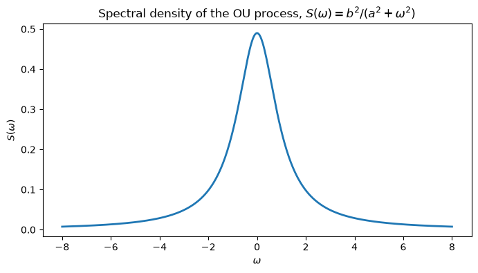
(a) Plot the spectral density \(S(\omega) = b^2/(a^2 + \omega^2)\).
(b) Verify property (iii) of the text numerically: the spectral density decomposes the variance, \(\frac{1}{2\pi}\int_{-\infty}^{\infty} S(\omega)\,d\omega = R(0) = b^2/(2a)\).
(c) Simulate a long OU path, form its periodogram (the sample analogue of the spectral density), and check that, after smoothing, it tracks \(S(\omega)\).
Solution to Exercise 8
a, b = 1.0, 0.7
S = lambda w: b**2 / (a**2 + w**2)

# (a) the spectral density
w = np.linspace(-8, 8, 400)
fig, ax = plt.subplots(figsize=(8, 4))
ax.plot(w, S(w), lw=2)
ax.set_xlabel(r'$\omega$'); ax.set_ylabel(r'$S(\omega)$')
ax.set_title(r'Spectral density of the OU process, $S(\omega)=b^2/(a^2+\omega^2)$')
plt.show()

# (b) variance decomposition
wfine = np.linspace(-1500, 1500, 3_000_001)
lhs = np.trapz(S(wfine), wfine) / (2 * np.pi)
print(f"(1/2π)∫S(w)dw = {lhs:.4f},   R(0) = b^2/2a = {b**2 / (2 * a):.4f}")
---------------------------------------------------------------------------
AttributeError                            Traceback (most recent call last)
Cell In[2], line 14
     10 plt.show()
     11
     12 # (b) variance decomposition
     13 wfine = np.linspace(-1500, 1500, 3_000_001)
---> 14 lhs = np.trapz(S(wfine), wfine) / (2 * np.pi)
     15 print(f"(1/2π)∫S(w)dw = {lhs:.4f},   R(0) = b^2/2a = {b**2 / (2 * a):.4f}")

File /opt/hostedtoolcache/Python/3.11.16/x64/lib/python3.11/site-packages/numpy/__init__.py:792, in __getattr__(attr)
    789     import numpy.char as char
    790     return char.chararray
--> 792 raise AttributeError(f"module {__name__!r} has no attribute {attr!r}")

AttributeError: module 'numpy' has no attribute 'trapz'
# (c) periodogram of a simulated OU path vs the theoretical spectrum
rng = np.random.default_rng(5)
dt, T = 0.05, 6000.0
steps = int(T / dt)
x = np.empty(steps); x[0] = 0.0
s = b * np.sqrt(dt)
for k in range(steps - 1):
    x[k + 1] = x[k] - a * x[k] * dt + s * rng.normal()
x = x[int(200 / dt):]            # burn-in
x = x - x.mean()

N = len(x)
freqs = np.fft.rfftfreq(N, d=dt) * 2 * np.pi      # angular frequencies
P = (dt / N) * np.abs(np.fft.rfft(x))**2          # periodogram

# band-average to tame the noise
nb = 200
edges = np.linspace(0, 8, nb + 1)
wc = 0.5 * (edges[1:] + edges[:-1])
Pb = np.array([P[(freqs >= edges[i]) & (freqs < edges[i + 1])].mean() for i in range(nb)])

fig, ax = plt.subplots(figsize=(8, 4))
ax.plot(wc, Pb, '.', alpha=0.5, label='periodogram (band-averaged)')
ww = np.linspace(0, 8, 400)
ax.plot(ww, S(ww), 'r-', lw=2, label=r'$S(\omega)=b^2/(a^2+\omega^2)$')
ax.set_xlabel(r'$\omega$'); ax.set_ylabel('spectral density')
ax.legend()
plt.show()
The numerical integral of \(S(\omega)/2\pi\) reproduces \(R(0) = b^2/(2a)\), and the smoothed periodogram of the simulated path follows the theoretical spectrum: most of the variance sits at low frequencies, with a \(1/\omega^2\) tail. The raw periodogram is very noisy, which is why we band-average. Exercise 9 shows why that step is not cosmetic.
Exercise 9
Why the periodogram must be smoothed. The band-averaging in part (c) above is not a refinement of the estimator; without it there is no consistency at all. This exercise makes that concrete.
Simulate the discretely sampled Ornstein–Uhlenbeck process (\(a=1\), \(b=0.7\), unit sampling), which is the AR(1) \(x_t = e^{-a}x_{t-1} + \eta_t\) with \(\sigma_\eta^2 = \frac{b^2}{2a}(1-e^{-2a})\), and form the periodogram \(I_N(\omega) = N^{-1}|\sum_t (x_t - \bar x)e^{-i\omega t}|^2\).
(a) Fix an interior frequency and, over many independent replications, tabulate the mean and standard deviation of \(I_N(\omega)\) for \(N = 128, 512, 2048\). The mean sits close to \(S(\omega)\) at every \(N\). The periodogram is asymptotically unbiased, and at this replication count the residual bias is not easily separated from Monte Carlo error. The point of the table is the other column: the standard deviation stays put at roughly \(S(\omega)\) itself, however large \(N\) becomes.
(b) Explain the result. \(I_N(\omega)\) is the squared modulus of a single Fourier coefficient, and that coefficient is asymptotically complex Gaussian with variance \(S(\omega)\), a fixed number of random quantities however long the record. Hence \(I_N(\omega)/S(\omega)\) is asymptotically \(\tfrac12\chi^2_2\), with mean \(1\) and variance \(1\), forever. Lengthening the record buys more frequencies, not more precision at any one of them.
(c) Now average over the \(m\) frequencies nearest \(\omega\) and watch the standard deviation fall like \(m^{-1/2}\). Consistency requires letting \(m\) grow with \(N\) while the bandwidth \(m/N\) shrinks. Those are the conditions \(b_N \to 0\) and \(Nb_N \to \infty\) of the spectral-window literature.
Solution to Exercise 9
rng = np.random.default_rng(0)
a, b = 1.0, 0.7
phi = np.exp(-a)
sig2 = (b**2/(2*a))*(1 - phi**2)

def periodograms(N, reps):
    """reps independent periodograms of an AR(1) record of length N."""
    out = np.empty((reps, N//2 + 1))
    for r in range(reps):
        e = rng.normal(0, np.sqrt(sig2), N + 500)
        x = np.zeros(N + 500)
        for t in range(1, N + 500):
            x[t] = phi*x[t-1] + e[t]
        x = x[500:]; x = x - x.mean()
        out[r] = np.abs(np.fft.rfft(x))**2 / N
    return out

print("   N     mean I     true S     s.d. I    s.d./S")
for N in [128, 512, 2048]:
    I = periodograms(N, 600)
    k = N//8                                   # a fixed interior frequency
    w = 2*np.pi*k/N
    Strue = sig2/np.abs(1 - phi*np.exp(-1j*w))**2
    print(f"{N:5d}   {I[:,k].mean():8.5f}   {Strue:8.5f}   {I[:,k].std():8.5f}   "
          f"{I[:,k].std()/Strue:6.3f}")
# (c) smoothing over m neighbouring ordinates: the s.d. falls like 1/sqrt(m)
N = 2048
I = periodograms(N, 600)
k = N//8
w = 2*np.pi*k/N
Strue = sig2/np.abs(1 - phi*np.exp(-1j*w))**2
print("   m   mean of smoothed I   s.d.    s.d./S   (1/sqrt(m) for comparison)")
for m in [1, 5, 25, 125]:
    sm = I[:, k-m//2 : k+m//2+1].mean(axis=1)
    print(f"{m:4d}   {sm.mean():14.5f}   {sm.std():7.5f}  {sm.std()/Strue:6.3f}"
          f"      {1/np.sqrt(m):6.3f}")
The first table is the point: the mean tracks \(S(\omega)\) but the standard deviation does not fall, staying at roughly \(S(\omega)\) as \(N\) increases sixteenfold. The periodogram is asymptotically unbiased and permanently noisy. In the second table, averaging \(m\) neighbouring ordinates cuts the standard deviation by very nearly \(m^{-1/2}\), as it would for \(m\) independent observations. Neighbouring periodogram ordinates are asymptotically independent.
That last clause is where the hidden assumption sits. Asymptotic independence across frequencies is a statement about fourth moments, not second, so nothing in this chapter establishes it; see A1. Ergodicity and the Consistent Estimation of Second Moments. The same appendix explains why consistency of the \(\hat R(\tau)\) feeding the periodogram is itself a fourth-moment question.