17. Discrete Sampling: The Folding Formula

We now confront the gap between the continuous time theory developed so far and the discretely sampled data we actually observe. The first question is what point-in-time sampling does to a process’s spectrum. The answer, the folding formula, drives the aliasing and identification problems that occupy the remainder of the book.

Let \(x(t)\) be a continuous time, covariance stationary stochastic process with autocovariogram \(R(\tau)\). Let \(x_j = x(jT)\) be a record of \(x\) sampled at the discrete points in time \(t = 0,\ \pm\, T,\ \pm\, 2T, \ldots,\) where \(T > 0\) is the sampling interval. The autocovariogram of the discrete data can be represented as a generalized function \(R^d(\tau)\) where

(119)\[ R^d(\tau) = \sum_{n=-\infty}^{\infty} R(nT)\, \delta(\tau - nT), \]

so that \(R^d(\tau)\) is a train of delta functions with mass \(R(nT)\) at \(\tau = 0,\ \pm\, T,\ \pm\, 2T, \ldots\,\). Equation (119) can also be represented as

\[ R^d(\tau) = R(\tau)\ S_T(\tau) \]

where

\[ S_T(\tau) = \sum_{n=-\infty}^{\infty} \delta(\tau - nT). \]

From (119), we can express the spectral density of the discrete sampled \(x_t\) as

(120)\[\begin{split}\begin{aligned} S^d(\omega) &= \int_{-\infty}^{\infty} R^d(\tau)\, e^{-i\omega\tau}\, d\tau \\ &= \sum_{n=-\infty}^{\infty} \int_{-\infty}^{\infty} R(\tau)\, e^{-i\omega\tau}\, \delta(\tau - nT)\, d\tau \\ &= \sum_{n=-\infty}^{\infty} R(nT)\, e^{-i\omega nT} \end{aligned}\end{split}\]

which is the discrete Fourier transform of the sequence \(R(nT),\ n = 0,\ \pm 1, \ldots\,\). It is shown by Papoulis [Papoulis, pp. 42–49] that the Fourier transform of the train of delta functions \(S_T(\tau) = \sum_{n=-\infty}^{\infty} \delta(\tau - nT)\) is given by

(121)\[\sum_{n=-\infty}^{\infty} \delta(\tau - nT) \leftrightarrow \omega_0 \sum_{n=-\infty}^{\infty} \delta(\omega - n\omega_0),\ \omega_0 = 2\pi/T.\]

Now notice that

(122)\[\omega_0 \sum_{n=-\infty}^{\infty} S(\omega - n\omega_0) = S(\omega) \ast \omega_0 \sum_{n=-\infty}^{\infty} \delta(\omega - n\omega_0).\]

By the multiplication property (property 7 of Table 2 of 8. Spectral Densities), multiplication in the time domain corresponds to convolution in the frequency domain divided by \(2\pi\), so the Fourier transform of \(R^d(\tau) = R(\tau)\, S_T(\tau)\) is

\[ \frac{1}{2\pi}\, S(\omega) \ast \omega_0 \sum_{n=-\infty}^{\infty} \delta(\omega - n \omega_0) = \frac{\omega_0}{2\pi} \sum_{n=-\infty}^{\infty} S(\omega - n \omega_0) = \frac{1}{T} \sum_{n=-\infty}^{\infty} S(\omega - n \omega_0), \]

since \(\omega_0/2\pi = 1/T\), the second equality being (122) read from right to left.

Because (120) identifies this transform as \(S^d(\omega)\), the spectral density of the discrete process \(x_j\) satisfies

(123)\[ S^d(\omega) = \frac{1}{T} \sum_{n=-\infty}^{\infty} S\!\left(\omega - n\, \frac{2\pi}{T}\right) \]

where \(S^d(\omega)\) is the spectral density of the discrete data and \(S(\omega)\) is the spectral density of the continuous time data. Equation (123) is known as the folding formula.

The folding formula is best read through the Cramér representation of 10. The Cramér Representation. There the process was exhibited as a superposition of mutually orthogonal frequency bands, the band \([c,\, d]\) contributing variance \(\frac{1}{\pi}\int_c^d S(\omega)\, d\omega\). Sampling does not destroy those bands: it wraps them, translating each by a multiple of \(\omega_0 = 2\pi/T\) onto the observable interval \([-\pi/T,\, \pi/T]\), where their variances simply add, the bands having been orthogonal. Equation (123) is that addition. The frequency \(\pi/T\), half the sampling rate, is the Nyquist frequency; everything above it is folded down on top of something below it.

The folding formula is therefore the engine of the aliasing problem: because infinitely many continuous time frequencies fold onto the same discrete frequency, the sampled spectrum cannot by itself recover the continuous one. The sampled data record only the sum of the folded bands, never the division of that sum among them. 21. Inferring a Continuous-Time System from Discrete-Time Data: An Appreciation of A. W. Phillips (1959) shows this is the same phenomenon as the multivalued \(\lambda = \log\mu\) in Phillips’s estimation problem; 22. The Dimensionality of the Aliasing Problem in Models with Rational Spectral Densities counts how many continuous time models survive the folding; and 23. Temporal Aggregation of Economic Time Series takes up the related distortions caused by time-averaging rather than point sampling.

Sampling can destroy ergodicity

One consequence of (123) concerns not what can be identified from sampled data but whether those data support estimation at all.

10. The Cramér Representation showed that a covariance stationary process is mean square ergodic, so that its time average converges to its ensemble mean, if and only if its spectral density carries no \(\delta\)-function at frequency zero. But sampling maps every continuous frequency \(\omega_1\) to the discrete frequency \(\omega_1\) modulo \(\omega_0 = 2\pi/T\). In particular,

an atom at any continuous frequency \(\omega_1 = 2\pi k/T\) folds onto discrete frequency zero.

A process can therefore be perfectly ergodic in continuous time and fail to be so once sampled. Take

\[ x(t) = A\cos(\omega_0 t) + B\sin(\omega_0 t), \qquad \omega_0 = \frac{2\pi}{T}, \]

with \(A, B\) uncorrelated, mean zero, variance \(\sigma^2\), so that \(R(\tau) = \sigma^2 \cos(\omega_0\tau)\). Its spectral density has \(\delta\)-functions at \(\pm \omega_0\) and none at the origin, so the continuous time average tends to zero: the process oscillates, and averaging over a long record averages it away. But sample at \(t = jT\), where \(\cos(\omega_0 jT) = \cos 2\pi j = 1\) and \(\sin(\omega_0 j T) = 0\), and

\[ x_j = A \qquad \text{for every } j : \]

a random constant, the non-ergodic process of 10. The Cramér Representation. An observer of the sampled data sees a series that never moves and can never learn \(\mu\), though the underlying process is in vigorous motion.

A deterministic seasonal at exactly the sampling frequency is thus harmless in continuous time and fatal in discrete time. This is the ergodic face of aliasing, complementary to the identification questions of 21. Inferring a Continuous-Time System from Discrete-Time Data: An Appreciation of A. W. Phillips (1959) and 22. The Dimensionality of the Aliasing Problem in Models with Rational Spectral Densities: those ask which continuous time models survive sampling, this asks whether the sampled record can estimate anything at all.

Exercises

The folding formula says that sampling a continuous time process at interval \(T\) produces a discrete time process whose spectral density is a sum of copies of the continuous spectrum, shifted by integer multiples of \(2\pi/T\) and superimposed (“folded”) onto the band \([-\pi/T, \pi/T]\). The frequency \(\pi/T\) is the Nyquist frequency. Power that the continuous process carries above the Nyquist frequency is not lost; it is aliased down into the observable band, distorting the discrete spectrum.

We illustrate this with the Ornstein–Uhlenbeck process of Chapters 7–8, whose continuous time spectral density is

\[ S(\omega) = \frac{b^2}{a^2 + \omega^2}, \qquad a, b > 0. \]

import numpy as np
import matplotlib.pyplot as plt

Exercise 21

Take \(a = 1\), \(b = 0.7\).

(a) Implement the folding formula

\[ S^d(\omega) = \frac{1}{T} \sum_{n=-\infty}^{\infty} S\!\left(\omega - n\,\frac{2\pi}{T}\right) \]

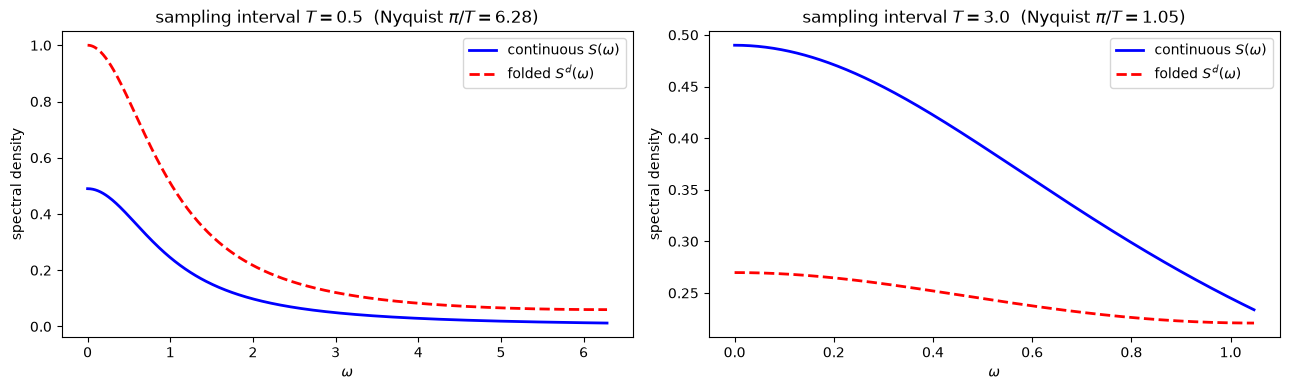
(truncating the sum at \(|n| \le n_{\max}\)). For a fast sampling rate (\(T = 0.5\)) and a slow one (\(T = 3\)), plot the continuous spectrum \(S(\omega)\) and the folded discrete spectrum \(S^d(\omega)\) on the observable band \([0, \pi/T]\). Comment on the aliasing.

(b) As an independent check, the discrete spectral density is also the discrete Fourier transform of the sampled autocovariance, \(S^d(\omega) = \sum_n R(nT)\,e^{-i\omega nT}\) with \(R(\tau) = \frac{b^2}{2a}e^{-a|\tau|}\) (equation (120)). Verify that this matches your folding-formula computation.

Solution to Exercise 21

a, b = 1.0, 0.7
S = lambda w: b**2 / (a**2 + w**2)

def folded_spectrum(w, T, nmax=80):
    """Discrete spectral density via the folding formula."""
    return sum(S(w - n * 2 * np.pi / T) for n in range(-nmax, nmax + 1)) / T

fig, axes = plt.subplots(1, 2, figsize=(13, 4))
for ax, T in zip(axes, [0.5, 3.0]):
    w_nyq = np.pi / T                      # Nyquist frequency
    w = np.linspace(0, w_nyq, 400)
    ax.plot(w, S(w), 'b-', lw=2, label=r'continuous $S(\omega)$')
    ax.plot(w, folded_spectrum(w, T), 'r--', lw=2, label=r'folded $S^d(\omega)$')
    ax.set_title(f'sampling interval $T={T}$  (Nyquist $\\pi/T={w_nyq:.2f}$)')
    ax.set_xlabel(r'$\omega$'); ax.set_ylabel('spectral density')
    ax.legend()
plt.tight_layout()
plt.show()

# (b) cross-check: folding formula vs DFT of the sampled autocovariance
def Sd_from_acov(w, T, nmax=4000):
    n = np.arange(-nmax, nmax + 1)
    Rn = (b**2 / (2 * a)) * np.exp(-a * np.abs(n * T))   # R(nT)
    return np.array([(Rn * np.exp(-1j * ww * n * T)).sum().real for ww in w])

T = 1.0
w = np.linspace(0, np.pi / T, 6)
print("folding formula :", np.round(folded_spectrum(w, T), 4))
print("DFT of R(nT)    :", np.round(Sd_from_acov(w, T), 4))

folding formula : [0.5299 0.3919 0.233  0.1552 0.1221 0.1129]
DFT of R(nT)    : [0.5302 0.3922 0.2333 0.1555 0.1224 0.1132]

With the fast sampling rate (\(T = 0.5\), Nyquist \(\approx 6.3\)) the OU spectrum has already decayed to nearly zero by the Nyquist frequency, so almost no power is folded back and \(S^d \approx S\) on the band. With the slow rate (\(T = 3\), Nyquist \(\approx 1.05\)) a substantial part of the continuous spectrum lives above the Nyquist frequency; it is aliased back into the band and the folded spectrum sits visibly above the continuous one. Part (b) confirms that the folding formula and the DFT of the sampled autocovariance agree to numerical precision, by two routes to the same discrete spectral density.

Exercise 22

A process that samples to a random constant. Take \(x(t) = A\cos(\omega_0 t) + B\sin(\omega_0 t)\) with \(A, B\) independent standard normals and \(\omega_0 = 2\pi/T\) for \(T = 1\).

(a) Plot a realization on \([0, 20]\) on a fine grid, and superimpose the values at the sampling instants \(t = 0, 1, \ldots, 20\). Confirm that the sampled values are all equal to the realized \(A\), while the continuous path oscillates with standard deviation close to \(1/\sqrt{2}\).

(b) Compute the running time average of the continuous path and confirm it tends to zero, while the running average of the sampled series is \(A\) at every horizon.

(c) Explain in terms of (123): where does the spectral mass of \(x\) sit, and where does sampling put it?

Solution to Exercise 22

rng = np.random.default_rng(3)
T = 1.0
w0 = 2*np.pi/T
A, B = rng.normal(), rng.normal()

t  = np.arange(0, 20, 0.002)          # fine grid: the continuous path
j  = np.arange(0, 21)                 # the sampling instants
xc = A*np.cos(w0*t) + B*np.sin(w0*t)
xs = A*np.cos(w0*j*T) + B*np.sin(w0*j*T)

print(f"realized A = {A:+.6f},  B = {B:+.6f}")
print(f"continuous path: mean {xc.mean():+.6f}, s.d. {xc.std():.6f}  (theory s.d. = {np.sqrt((A**2+B**2)/2):.6f})")
print(f"sampled values : {np.unique(np.round(xs, 12))}   <- a single number, equal to A")
print(f"running mean of sampled series at j=5, 20: {xs[:5].mean():+.6f}, {xs[:20].mean():+.6f}")

realized A = +2.040919,  B = -2.555665
continuous path: mean -0.000000, s.d. 2.312658  (theory s.d. = 2.312658)
sampled values : [2.04091912]   <- a single number, equal to A
running mean of sampled series at j=5, 20: +2.040919, +2.040919

fig, ax = plt.subplots(figsize=(11, 4))
ax.plot(t, xc, lw=0.9, color='C0', label='continuous path $x(t)$')
ax.plot(j, xs, 'o', ms=7, color='C3', label='sampled $x_j$: every value equals $A$')
ax.axhline(A, color='C3', ls=':', lw=1)
ax.axhline(0, color='k', lw=0.5)
ax.set_xlim(0, 20); ax.set_xlabel('$t$'); ax.set_ylabel('$x$')
ax.set_title('A process that is mean square ergodic in continuous time, and not after sampling')
ax.legend(loc='upper right', fontsize=9)
plt.show()

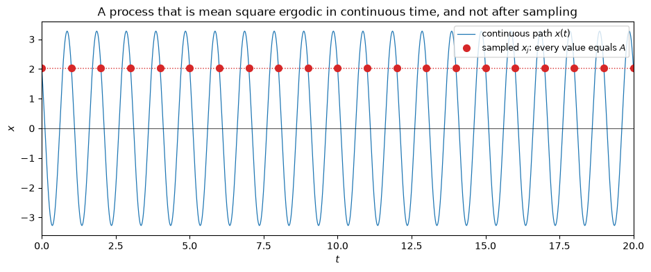
The spectral mass of \(x\) sits entirely at \(\pm \omega_0\), away from the origin, so the continuous time average washes it out. Sampling at interval \(T = 2\pi/\omega_0\) folds those two atoms onto discrete frequency zero, and what had been an oscillation becomes a constant. The sampled record contains one number, repeated; no length of record will reveal the mean.