Preliminary Concepts[1]

A stochastic process is a collection of random variables, a collection indexed by a variable \(t\). In our work, we shall regard \(t\) as time and will require \(t\) to be an integer, so that we shall be working in discrete time. Thus, the stochastic process \(y_t\) is a collection of random variables \(\ldots, y_{-1}, y_0, y_1, y_2, \ldots\), there being one random variable for each point in time \(t\) belonging to the set \(T\), which in our case is the set of integers. Alternatively, on each “drawing”, we draw an entire sequence \(\{y_k\}_{k=-\infty}^{\infty}\). We are interested in the probability distribution of such sequences. A single drawing of a sequence \(\{y_k\}\) is called a realization of the stochastic process \(y_t\).

We shall characterize the probability law governing the collection of random variables that make up the stochastic process by the list of means of \(y_t\) and by the covariances between the \(y\)’s at different points in time. (For a stochastic process that obeys the normal probability law, these parameters completely characterize the probability distribution. Even where \(y\) is not normal, the first and second moments contain much useful information, enough information to characterize the linear structure of the process.) In particular, the mean of the process \(y_t\) is

\[ Ey_t = \mu_t, \quad t \in T, \]

where \(E\) is the mathematical expectation operator. The covariances are given by

\[ E[(y_t-\mu_t)(y_s-\mu_s)] = \sigma_{t,s}. \]

A stochastic process is said to be wide-sense stationary (or covariance stationary or second-order stationary) if \(\mu_t\) is independent of \(t\) and if \(\sigma_{t,s}\) depends only on \(t-s\). We shall henceforth deal with such stationary processes. The first and second moments of a stationary process are summarized by the mean \(\mu\) and the covariogram \(c(\tau)\) defined by

\[ E[(y_t-\mu)(y_s-\mu)] = \sigma_{t,s} = E[(y_t-\mu)(y_{t-\tau}-\mu)] = \sigma_{t,t-\tau} \equiv c(\tau), \]

where \(\tau = t-s\). The covariogram is easily verified to be symmetric, i.e., \(c(\tau) = c(-\tau)\), and to obey \(c(0) \geq |c(\tau)|\) for all \(\tau\), this inequality being an implication of the Schwarz inequality.

To find further restrictions on the covariogram, let \(x_t\) be a covariance stationary stochastic process with mean zero and covariogram \(c(\tau)\). Consider forming a weighted sum of all \(x\)’s at different dates

\[ y = \sum_{j=1}^n a_j x_{t_j}, \]

where the \(a_j\) are fixed numbers and \(t_1, \ldots, t_n\) are integers. We must require that the random variables \(y\) have nonnegative variance, so that

\[ Ey^2 = E\!\left(\sum_{j=1}^n a_j x_{t_j} \sum_{k=1}^n a_k x_{t_k}\right) = \sum_{j=1}^n \sum_{k=1}^n a_j a_k\, E x_{t_j} x_{t_k} = \sum_{j=1}^n \sum_{k=1}^n a_j a_k\, c(t_k - t_j) \geq 0. \]

This last inequality is required to hold for any \(n\), any list of \(a_j\), and any selection of \((t_1, t_2, \ldots, t_n)\). A sequence \(c(\tau)\) that satisfies this condition is said to be nonnegative definite. The condition that \(c(\tau)\) be nonnegative definite is a necessary and sufficient condition for a sequence \(c(\tau)\) to be the covariogram of a well-defined stochastic process.[2]

White Noise

A basic building block is the serially uncorrelated random process \(\epsilon_t\), which satisfies:

(156)\[\begin{split}E(\epsilon_t) = 0 \quad \text{for all } t, \\ E(\epsilon_t^2) = \sigma_\epsilon^2 \quad \text{for all } t, \\ E(\epsilon_t \epsilon_{t-s}) = 0 \quad \text{for all } t \text{ and all } s \neq 0.\end{split}\]

This process is (wide-sense) stationary, each variate being uncorrelated with itself lagged \(s = \pm 1, \pm 2, \ldots\) times, and is said to be serially uncorrelated. The process is also often referred to as “white noise.” As we shall see, such a white-noise process can be viewed as the basic building block for a large class of stationary stochastic processes.

Moving Average Processes and the Covariance Generating Function

To illustrate how the white-noise process \(\epsilon_t\) can be used to build up more complicated processes, consider the random process \(y_t\):

(157)\[y_t = \sum_{j=0}^{\infty} b_j \epsilon_{t-j} = B(L)\epsilon_t,\]

where \(B(L) = \sum_{j=0}^{\infty} b_j L^j\), and where we assume \(\sum_{j=0}^{\infty} b_j^2 < \infty\), a requirement needed to assure that the variance of \(y\) is finite. We assume that the \(\epsilon\) process is “white” and thus satisfies properties (156). Equation (157) says that the \(y\) process is a one-sided moving sum of a white-noise process \(\epsilon\).

We seek the covariogram of the \(y\) process, i.e., the values of \(c_y(k) = E(y_t y_{t-k})\) for all \(k\). It will be convenient to obtain the covariance generating function \(g_y(z)\), defined by

(158)\[g_y(z) = \sum_{k=-\infty}^{\infty} c_y(k)\, z^k.\]

The coefficient on \(z^k\) in (158) is the \(k\)th lagged covariance \(c_y(k)\).

First notice that taking mathematical expectation on both sides of (157) gives

\[ E(y_t) = \sum_{j=0}^{\infty} b_j E(\epsilon_{t-j}) = 0 \quad \text{for all } t. \]

It therefore follows that \(c_y(k) = E\{(y_t - Ey_t)(y_{t-k} - Ey_{t-k})\} = Ey_t y_{t-k}\) for all \(k\). Since the \(\{\epsilon_t\}\) process is serially uncorrelated, it follows that

\[ Ey_t y_{t-k} = E\!\left( \sum_{j=-\infty}^{\infty} b_j \epsilon_{t-j} \sum_{h=-\infty}^{\infty} b_h \epsilon_{t-k-h} \right) = \sigma_\epsilon^2 \sum_{j=-\infty}^{\infty} b_j b_{j-k}, \]

since only for \(j = k+h\) (or \(h = j-k\)) is \(E\epsilon_{t-j}\epsilon_{t-k-h}\) nonzero and equal to \(\sigma_\epsilon^2\). We have permitted the \(j\) and \(h\) indexes to run over negative values, though in our case \(b_j = 0\) for \(j < 0\). (The formula is correct even if \(b_j \neq 0\) for \(j < 0\).) The covariance generating function is then

\[ g_y(z) = \sigma_\epsilon^2 \sum_{k=-\infty}^{\infty} z^k \sum_{j=-\infty}^{\infty} b_j b_{j-k} = \sigma_\epsilon^2 \sum_{j=-\infty}^{\infty} \sum_{k=-\infty}^{\infty} b_j b_{j-k}\, z^k. \]

Letting \(h = j-k\) so that \(k = j-h\), we have

\[ g_y(z) = \sigma_\epsilon^2 \sum_{j=-\infty}^{\infty} \sum_{h=-\infty}^{\infty} b_j b_h\, z^{j-h} = \sigma_\epsilon^2 \sum_{j=-\infty}^{\infty} b_j z^j \sum_{h=-\infty}^{\infty} b_h z^{-h}. \]

The last equation gives the convenient expression

(159)\[g_y(z) = \sigma_\epsilon^2\, B(z^{-1})\, B(z),\]

where \(B(z^{-1}) = \sum_{j=-\infty}^{\infty} b_j z^{-j}\) and \(B(z) = \sum_{j=-\infty}^{\infty} b_j z^j\). Equation (159) gives the covariance generating function \(g_y(z)\) in terms of the \(b_j\) and the variance \(\sigma_\epsilon^2\) of the white noise \(\epsilon\).

First-Order Autoregressive Process

To take an example that illustrates the usefulness of (159), consider the first-order process

(160)\[y_t = \lambda y_{t-1} + \epsilon_t \quad\text{or}\quad y_t = \frac{1}{1-\lambda L}\,\epsilon_t = \sum_{i=0}^{\infty} \lambda^i \epsilon_{t-i}, \quad |\lambda| < 1,\]

where, as always, \(\epsilon\) is a white-noise process with variance \(\sigma_\epsilon^2\). We have

\[ B(L) = \frac{1}{1-\lambda L}, \quad B(z) = \frac{1}{1-\lambda z} = 1 + \lambda z + \lambda^2 z^2 + \cdots, \quad B(z^{-1}) = \frac{1}{1-\lambda z^{-1}} = 1 + \lambda z^{-1} + \lambda^2 z^{-2} + \cdots. \]

(Thus, \(B(z)\) is found by replacing \(L\) in \(B(L)\) by \(z\).) So applying (159) we have

(161)\[g_y(z) = \sigma_\epsilon^2 \left(\frac{1}{1-\lambda z^{-1}}\right)\!\left(\frac{1}{1-\lambda z}\right).\]

From our experience with difference equations we know that the expression (161) can be written as a sum

(162)\[g_y(z) = \frac{k_1 \sigma_\epsilon^2}{1-\lambda z} + \frac{k_2 \sigma_\epsilon^2 z^{-1}}{1-\lambda z^{-1}},\]

where \(k_1\) and \(k_2\) are certain constants. To find out what the constants must be, notice that (162) implies

\[ g_y(z) = \sigma_\epsilon^2 k_1 (1 + \lambda z + \lambda^2 z^2 + \cdots) + \sigma_\epsilon^2 k_2 (z^{-1} + \lambda z^{-2} + \lambda^2 z^{-3} + \cdots), \]

so that \(c_y(0) = k_1 \sigma_\epsilon^2\) and \(c_y(1) = \sigma_\epsilon^2 \lambda k_1 = \sigma_\epsilon^2 k_2 = c_y(-1)\). By direct computation using (160) we note that

\[ Ey_t^2 = \sum_{i=0}^{\infty} \lambda^{2i} E\epsilon_t^2 = \frac{\sigma_\epsilon^2}{1-\lambda^2}, \qquad Ey_t y_{t-1} = E \sum_{i=0}^{\infty} \lambda^i \epsilon_{t-i} \sum_{j=1}^{\infty} \lambda^{j-1} \epsilon_{t-j} = \sigma_\epsilon^2 \lambda \sum_{i=1}^{\infty} \lambda^{2(i-1)} = \frac{\lambda \sigma_\epsilon^2}{1-\lambda^2}. \]

So for (162) to be correct, we require that

\[ \sigma_\epsilon^2 \left[ \frac{1/(1-\lambda^2)}{1-\lambda z} + \frac{z^{-1}(\lambda/(1-\lambda^2))}{1-\lambda z^{-1}} \right] = \sigma_\epsilon^2 \frac{1}{1-\lambda^2} \left[\frac{1 - \lambda z^{-1} + \lambda z^{-1} - \lambda^2}{(1-\lambda z)(1-\lambda z^{-1})}\right] = \frac{\sigma_\epsilon^2}{(1-\lambda z)(1-\lambda z^{-1})}, \]

so that (161) and (162) are equivalent.

Expression (162) is the more convenient of the two since it yields quite directly

\[ g_y(z) = \sigma_\epsilon^2 \frac{1}{1-\lambda^2} \left[\frac{1}{1-\lambda z} + \frac{\lambda z^{-1}}{1-\lambda z^{-1}}\right] = \sigma_\epsilon^2 \frac{1}{1-\lambda^2} \left[\{1 + \lambda z + \lambda^2 z^2 + \cdots\} + \{\lambda z^{-1} + \lambda^2 z^{-2} + \lambda^3 z^{-3} + \cdots\}\right]. \]

Thus, we have that for the first-order Markov process (160)

\[ c_y(k) = \frac{\sigma_\epsilon^2}{1-\lambda^2}\,\lambda^{|k|}, \qquad k = 0, \pm 1, \pm 2, \ldots \]

The covariance declines geometrically with increases in \(|k|\). We require \(|\lambda| < 1\) in order that the \(y\) process have a finite variance.

The Yule-Walker Equation

To get this result more directly, write the stochastic difference equation \(y_t = \lambda y_{t-1} + \epsilon_t\), then multiply \(y_t\) by \(y_{t-k}\), \(k > 0\), to obtain

\[ y_t y_{t-k} = \lambda y_{t-1} y_{t-k} + \epsilon_t y_{t-k}. \]

Taking expected values on both sides and noting that \(E\epsilon_t y_{t-k} = 0\) gives the famous Yule-Walker equation

\[ E(y_t y_{t-k}) = \lambda E(y_{t-1} y_{t-k}) \quad\text{or}\quad c_y(k) = \lambda c_y(k-1), \qquad k > 0, \]

which implies the solution

\[ c_y(k) = \lambda^k c_y(0), \qquad k > 0. \]

From symmetry of covariograms, it then follows that \(c_y(k) = \lambda^{|k|} c_y(0)\) for all \(k\). Notice that the covariogram obeys the solution of the nonrandom part of the difference equation with initial condition \(c_y(0)\).

Second-Order Autoregressive Process

As a second example, consider the second-order process

(163)\[y_t = \frac{1}{(1-\lambda_1 L)(1-\lambda_2 L)}\,\epsilon_t, \qquad |\lambda_1| < 1,\; |\lambda_2| < 1,\; \lambda_1 \neq \lambda_2,\]

where \(\epsilon_t\) is white noise with variance \(\sigma_\epsilon^2\). Multiply both sides of (163) by \((1-\lambda_1 L)(1-\lambda_2 L)\) to get

(164)\[y_t = t_1 y_{t-1} + t_2 y_{t-2} + \epsilon_t,\]

where \(t_1 = \lambda_1 + \lambda_2\) and \(t_2 = -\lambda_1 \lambda_2\). Multiply (164) by \(y_{t-k}\) for \(k > 0\) to get

\[ y_t y_{t-k} = t_1 y_{t-1} y_{t-k} + t_2 y_{t-2} y_{t-k} + \epsilon_t y_{t-k}. \]

Since \(E\epsilon_t y_{t-k} = 0\), we have

\[ E(y_t y_{t-k}) = t_1 E(y_{t-1} y_{t-k}) + t_2 E(y_{t-2} y_{t-k}), \qquad k > 0, \]

which shows that \(c_y(k)\) obeys the difference equation (the Yule-Walker equation)

(165)\[c_y(k) = t_1\, c_y(k-1) + t_2\, c_y(k-2).\]

So the covariogram of a second- (\(n\)th-) order process obeys the solution to the deterministic second- (\(n\)th-) order difference equation examined above. In particular, corresponding to (165) we consider the polynomial

(166)\[1 - t_1 k - t_2 k^2 = 0,\]

which has roots \(1/\lambda_1\) and \(1/\lambda_2\). (We know that \(1 - t_1 k - t_2 k^2 = (1-\lambda_1 k)(1-\lambda_2 k)\), with roots \(1/\lambda_1\) and \(1/\lambda_2\).) Alternatively, multiply (166) by \(k^{-2}\) to obtain

(167)\[k^{-2} - t_1 k^{-1} - t_2 = 0, \qquad x^2 - t_1 x - t_2 = 0 \;\text{ where }\; x = k^{-1}.\]

Notice that the roots of (167) are the reciprocals of the roots of (166), so \(\lambda_1\) and \(\lambda_2\) are roots of (167).

The solution to the deterministic difference equation (165) is, as we have seen,

(168)\[c_y(k) = \lambda_1^k z_0 + \lambda_2^k z_1, \qquad k \geq 0,\]

where \(z_0\) and \(z_1\) are certain constants chosen to make \(c_y(0)\) and \(c_y(1)\) equal the proper quantities. If roots \(\lambda_1\) and \(\lambda_2\) are complex, we know from our work with deterministic difference equations and from the symmetry of covariograms that

(169)\[c_y(k) = 2p\, r^k \cos(\omega k) \qquad\text{or}\qquad c_y(k) = c_y(0)\, r^k \cos(\omega k),\]

where \(\lambda_1 = re^{i\omega}\) and \(\lambda_2 = re^{-i\omega}\). According to (169), the covariogram displays damped (we require \(r < 1\)) oscillations with angular frequency \(\omega\). A complete cycle occurs as \(\omega k\) goes from zero (\(k = 0\)) to \(2\pi\) (\(k = 2\pi/\omega\), if that is possible). The restrictions on \(t_1\) and \(t_2\) needed to deliver complex roots and so an oscillatory covariogram can be read directly from Figure 1 of Chapter IX.

Figure 1b displays a realization of a second-order process for values of \(t_1\) and \(t_2\) for which the roots are complex. Notice the tendency of this series to cycle, but with a periodicity that is somewhat variable from cycle to cycle. Figure 1a reports a realization of a first-order autoregressive process.

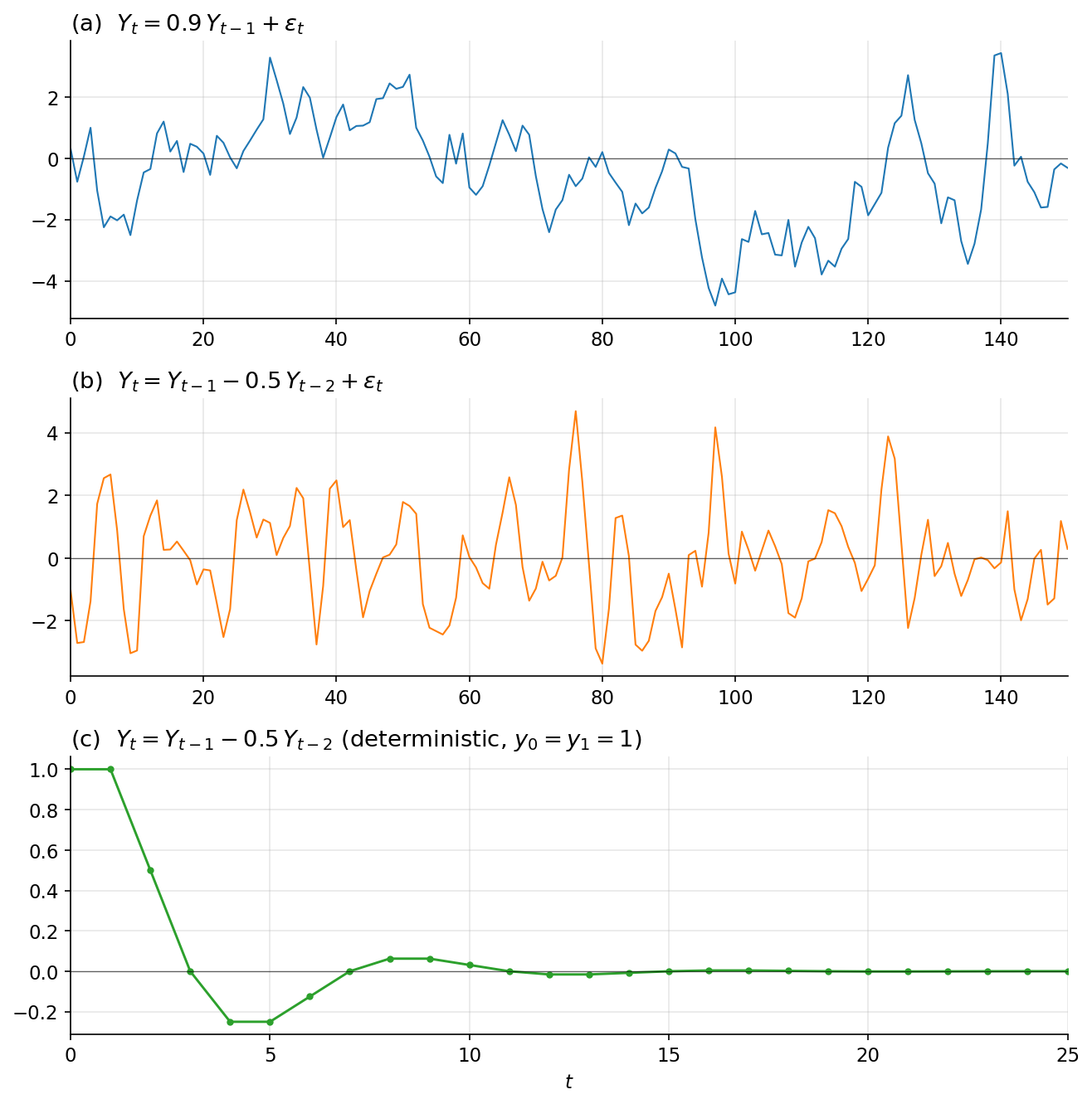
Fig. 5 Figure 1. (a) Realization of a first-order AR process (160) with \(\lambda = 0.9\). (b) Realization of a second-order AR process (164) with complex roots. (c) Solution of the deterministic part of the same second-order difference equation with initial conditions \(y_0 = y_1 = 1\). Generated by code/fig1_ar_realizations.py.

The foregoing suggests one tentative definition of a cycle in a single series: a series may be said to possess a “cycle” if its covariogram is characterized by (damped) oscillations. The typical “length” of the cycle can be measured by \(2\pi/\omega\), where \(\omega\) is the angular frequency associated with the damped oscillations in the covariogram (e.g., see (169)). To be labeled a business cycle the cycle should exceed a year in length. (Cycles of one year in length are termed seasonals.) We advance this only as a tentative definition of a cycle, and put off for a while discussing its adequacy.

---

[1]

The reader is assumed to be familiar with complex variables. The chapter on complex variables in Allen (1960) is a good place to start. See Churchill et al. (1974) for a more extensive treatment.

[2]

The conditions turn out to be equivalent with the condition that the spectral density of \(x\) be nonnegative, a condition which also in effect stems from the requirement that the variance of every linear combination of \(x\)’s at different points in time be nonnegative.