Deriving the Moving Average Representation

The univariate prediction formulas given above assume that one has in hand a moving average representation for the covariance stationary stochastic process \(x_t = d(L)\epsilon_t\), in which \(\epsilon_t\) lies in the linear space spanned by current and lagged \(x_t\)’s. Suppose that one starts with a covariogram \(c(\tau)\) of \(x_t\) and wishes to obtain such a moving average representation. We show how to accomplish this, beginning with a special case of a first-order moving average process.

Suppose that \(c(\tau) = 0\) for \(|\tau| \geq 2\). We seek a first order moving average process

(250)\[x_t = d_0 \epsilon_t + d_1 \epsilon_{t-1}\]

where \(\epsilon_t\) is a white noise that can be expressed as a square summable linear combination of \(\{x_t, x_{t-1}, \ldots\}\). If representation (250) is correct, then we must have

(251)\[\begin{split}\begin{aligned} c(0) &= (d_0^2 + d_1^2)\sigma_\epsilon^2 \\ c(1) &= d_0 d_1 \sigma_\epsilon^2. \end{aligned}\end{split}\]

The idea is now to solve (251) for \((d_0, d_1, \sigma_\epsilon^2)\) as a function of \(c(0), c(1)\). It is evident that we can solve (251) while normalizing by setting \(d_0 = 1\). Solving the second equation for \(\sigma_\epsilon^2 = c(1)/d_1\) and substituting into the first equation of (251) gives the “Euler Equation”

\[ d_1^{-1} - \frac{c(0)}{c(1)} + d_1 = 0 \]

We call this an Euler Equation because the coefficient on \(d_1^{-1}\) equals that on \(d_1\). To solve this equation, we can express it as

(252)\[\left(1 - \frac{c(0)}{c(1)}d_1 + d_1^2\right) = 0.\]

We seek to solve this for values of \(d_1\). The roots of (252) come in a reciprocal pair. As in Chapter IX, let \(\lambda\) be one root and \(\lambda^{-1}\) be the other. Then we want to solve

(253)\[\left(1 - \frac{c(0)}{c(1)}d_1 + d_1^2\right) = (1 - \lambda d_1)\left(1 - \frac{1}{\lambda}d_1\right).\]

Equating powers of \(d_1\), we find that we must solve the equation

\[ \lambda + \frac{1}{\lambda} = \frac{c(0)}{c(1)}. \]

A version of Figure 4 of Chapter IX can be used to solve this equation graphically (see Figure 7). Since \(|\lambda + 1/\lambda|\geq 2\), it follows that we must have \(|c(0)/c(1)|\geq 2\), or \(2|c(1)|\leq c(0)\) in order that there exist real values of \(d_1\) that solve (252).[1]

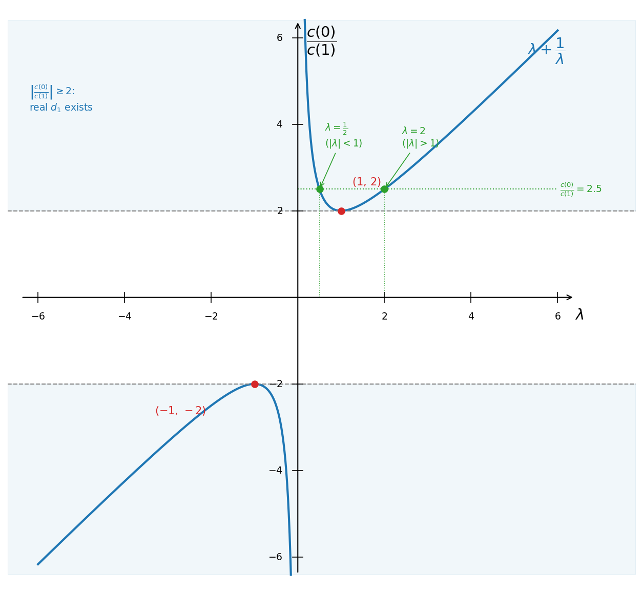
Fig. 16 Figure 7. Factoring the “Euler equation” of a first-order moving average: the graph of \(\lambda + 1/\lambda\) versus \(\lambda\). Because \(|\lambda + 1/\lambda| \geq 2\), with the minimum \(2\) at \(\lambda = 1\) and the maximum \(-2\) at \(\lambda = -1\) (red dots), a real root exists only when the ratio \(c(0)/c(1)\) lands in the shaded region \(|c(0)/c(1)| \geq 2\) — equivalently \(2|c(1)| \leq c(0)\). Each admissible ratio is met by a reciprocal pair \(\lambda\) and \(1/\lambda\) (the worked example \(c(0)/c(1) = 2.5\) gives \(\lambda = \tfrac12\) and \(\lambda = 2\)): one inside the unit circle, the fundamental choice, and one outside. Generated by code/fig7_euler_factoring.py.

Alternatively, applying the quadratic formula to (252), we obtain

\[ d_1 = \frac{\frac{c(0)}{c(1)} \pm \sqrt{\left(\frac{c(0)}{c(1)}\right)^2 - 4}}{2} \]

Again, we require that \(2|c(1)|\leq c(0)\) in order for a real solution to exist.

Once \(d_1\) is found, \(\sigma_\epsilon^2\) is found from the equation \(\sigma_\epsilon^2 = c(1)/d_1\).

We have that for \(2|c(1)|\leq c(0)\), there is a pair of solutions, one with \(|d_1|>1\), the other with \(|d_1|<1\). Thus, there are two representations of the form (250). Notice that from the formula \(\sigma_\epsilon^2 = c(1)/d_1\), the solution with the smaller absolute value \(d_1\) (the one that is less than unity in absolute value) is the one associated with the larger error variance. This suggests that associated with our two solutions are distinct \(\epsilon_t\) processes. Our calculations so far have not yet built in the requirement that \(\epsilon_t\) lies in the space spanned by current and lagged \(x_t\)’s. This requirement is imposed by selecting the solution with \(|d_1|<1\). Since

\[ x_t = \epsilon_t + d_1\epsilon_{t-1} \]

we have

\[ (1 + d_1 L)\epsilon_t = x_t \]

For \(|d_1|<1\), we have that \(\epsilon_t\) can be expressed as a square summable linear combination of current and lagged \(x_t\)’s:

(254)\[\epsilon_t = \sum_{j=0}^\infty(-d_1)^j x_{t-j}\]

However, when \(|d_1|>1\), the right side of the representation (254) is not square summable. When \(|d_1|>1\), the \(\epsilon_t\) in (250) lies in the linear space spanned by square summable linear combinations of future \(x_t\)’s and can be expressed as

\[ \epsilon_t = \sum_{j=1}^\infty (-1)^{j-1}\left(\frac{1}{d_1}\right)^j x_{t+j}. \]

Thus, to obtain the representation in which \(\epsilon_t\) lies in the linear space spanned by \(\{x_t, x_{t-1}, \ldots\}\), we select \(|d_1|<1\). Since \(\sigma_\epsilon^2 = c(1)/d_1\), this selection results in selecting from among moving average representations that satisfy (251) the one for which \(\sigma_\epsilon^2\) is maximal. For the representation chosen in this way, \(\sigma_\epsilon^2\) is the variance of \((x_t - P[x_t | x_{t-1}, x_{t-2}, \ldots])\). The white noise process \(\epsilon_t\) chosen by this procedure is said to be fundamental white noise for \(x_t\), meaning that it equals the process of one-step ahead errors in predicting \(x_t\) from its own past values.[2]

---

[1]

The spectral density for this \(x_t\) process is given by \(g_x(e^{-i\omega}) = c(0) + 2 c(1)\cos \omega\). We require that \(2|c(1)| < c(0)\) in order that the spectral density be nonnegative, or equivalently, in order that \(c(\tau)\) be a nonnegative definite sequence.

[2]

One sometimes encounters an alternative condition that serves to select the moving average representation with a fundamental white noise. This is the “minimum phase condition” which in our example requires that the solution of (251) be selected in which the phase of \(d(e^{-i\omega}) = 1 + d_1 e^{-i\omega}\) is smallest. For our example, the phase of \(d(e^{-i\omega})\) is given by \(\theta(\omega) = \tan^{-1}(-d_1 \sin \omega/(1 + d_1 \cos \omega))\). For low frequency, this is minimized in absolute value when the solution with \(|d_1| < 1\) is selected.