Chapter IX — Difference Equations and Lag Operators[1]#
Linear difference equations underlie much work in macroeconomics and applied economic dynamics. Lag operators provide a powerful tool for solving systems of linear difference equations, and for gaining insights about their structure. Lag operators constitute a language which much of macroeconomics and dynamic econometrics takes for granted. This chapter provides an introduction to the analysis of nonstochastic difference equations via lag operators. While a variety of economic examples occur in this chapter, additional examples continue to occur throughout the remainder of this book.
1. Lag Operators#
The backward shift or lag operator is defined by
Multiplying a variable \(X_t\) by \(L^n\) thus gives the value of \(X\) shifted back \(n\) periods. Notice that if \(n < 0\) in (1), the effect of multiplying \(X_t\) by \(L^n\) (more precisely, the effect of “operating on \(X_t\) with \(L^n\)”) is to shift \(X\) forward in time by \(-n\) periods.[2] This language is loose. Actually, we are starting out with a sequence \(\{X_t\}_{t=-\infty}^{\infty}\) which associates a real number \(X_t\) with each integer \(t\). We are operating on the sequence \(\{X_t\}\) with the operator \(L^n\) to obtain the new sequence \(\{y_t\}_{t=-\infty}^{\infty} = \{X_{t-n}\}_{t=-\infty}^{\infty}\). Formally, the operator \(L^n\) maps one sequence into another sequence.
We shall consider polynomials in the lag operator
where the \(a_j\)’s are constants and \(L^0 \equiv 1\). Operating on \(X_t\) with \(A(L)\) yields a moving sum of \(X\)’s:
It is generally convenient to work with polynomials \(A(L)\) that are “rational,” meaning that they can be expressed as the ratio of two (finite order) polynomials in \(L\):
where
where the \(b_j\) and \(c_j\) are constants. Assuming that \(A(L)\) is rational amounts to imposing a more economical and restrictive parametrization on the \(a_j\).
To take the simplest example of a rational polynomial in \(L\), consider[3]
For the scalar \(|C| < 1\), we know that
This suggests treating \(\lambda L\) of (2) exactly like the \(C\) of (3) to get
an expansion which is sometimes only “useful” so long as \(|\lambda| < 1\). To motivate the equality (4), assume that \(|\lambda| < 1\) and operate on both sides of (4) with \(1 - \lambda L\) to obtain
The reason that we say that (4) is sometimes “useful” only if \(|\lambda| < 1\) derives from the following argument. We intend often to multiply \(1/(1 - \lambda L)\) by \(X_t\) to obtain the infinite moving sum
Consider this sum for a path of \(X\) that is constant over time, so that \(X_{t-i} = \bar{X}\) for all \(i\) and all \(t\). Then the sum (5) becomes
The sum \(\sum_{i=0}^{\infty} \lambda^i\) equals \(1/(1 - \lambda)\) if \(|\lambda| < 1\). But if \(|\lambda| \geq 1\) that sum is unbounded, being \(+\infty\) if \(\lambda \geq 1\). We shall sometimes (though not always) be applying the polynomial in the lag operator (4) in situations in which it is appropriate to go infinitely far back in time; and we sometimes find it necessary to insist that in such cases the infinite sum in (5) exist where \(X\) has been constant through time. This is what leads to the requirement sometimes imposed that \(|\lambda| < 1\) in (4). As we shall see, however, in standard analyses of difference equations, which take the starting point of all processes as some point only finitely far back into the past, the requirement that \(|\lambda| < 1\) need not be imposed in (4).
It is useful to note that there is an alternative expansion for the “geometric” polynomial \(1/(1 - \lambda L)\). For notice that formally
an expansion which is especially “useful” where \(|\lambda| > 1\), i.e., where \(|1/\lambda| < 1\). So (6) implies that
which shows \((1/(1 - \lambda L))X_t\) to be a geometrically declining weighted sum of future values of \(X\). Notice that for this infinite sum to be finite for a constant time path \(X_{t+i} = \bar{X}\) for all \(i\) and \(t\), the series \(-\sum_{i=1}^{\infty}(1/\lambda)^i\) must be convergent, which requires that \(|1/\lambda| < 1\).
More generally, let \(\{x_t\}_{t=-\infty}^{\infty}\) be any bounded sequence of real numbers, i.e., for some \(M > 0\), \(|x_t| < M\) for all \(t\). Then applying the operator \(1/(1 - \lambda L)\) to the sequence \(\{x_t\}_{t=-\infty}^{\infty}\) can be taken to give either the sequence \(\{y_t\}_{t=-\infty}^{\infty}\) where
or the sequence \(\{z_t\}_{t=-\infty}^{\infty}\) where
In general, \(\{y_t\}\) is a bounded sequence if \(|\lambda| < 1\), while \(\{z_t\}\) is a bounded sequence if \(|\lambda| > 1\). In many (though not all) contexts, we want application of \((1 - \lambda L)^{-1}\) to map all bounded sequences into bounded sequences, so that we choose the “backward” expansion if \(|\lambda| < 1\) and the forward expansion if \(|\lambda| > 1\).
To illustrate how polynomials in the lag operator can be manipulated, consider the difference equation
where \(X_t\) is an exogenous variable and \(Y_t\) is an endogenous variable and \(\lambda \neq 1\). Here, \(X_t\) is a sequence of real numbers \(t = \cdots, -1, 0, 1, 2, \ldots\). Write the above equation as
Operating on both sides of this equation by \((1 - \lambda L)^{-1}\) gives
since \(a/(1 - \lambda L) = a\sum_{i=0}^{\infty}\lambda^i = a/(1 - \lambda)\). Here \(c\) is any constant. The reason that we must include the term \(c\lambda^t\) in (8) is that for any constant \(c\), \((1 - \lambda L)c\lambda^t = c\lambda^t - c\lambda\lambda^{t-1} = 0\).[4] Therefore, it follows that application of \(1 - \lambda L\) to both sides of (8) gives Equation (7) once again. Consequently, (8) is the general “solution” of the difference equation (7) and describes the entire time path of \(Y\) associated with a given time path of \(X\). In order to get a “particular solution” we must be able to tie down the constant \(c\). This requires an additional bit of information in the form of a specified value of \(Y_t\) at some particular time or some conditions on the path of \(\{Y_t\}\) such as boundedness. Notice that for the \(Y_t\) defined by (8) to be finite, \(\lambda^i X_{t-i}\) must be “small” for large \(i\). More precisely, we require
For the case of \(X\) constant for all time, \(X_{t-i} = \bar{X}\) all \(i\) and \(t\), this condition requires \(|\lambda| < 1\). Notice also that the infinite sum \(a\sum_{i=0}^{\infty}\lambda^i\) in (8) is finite only if \(|\lambda| < 1\), in which case it equals \(a/(1 - \lambda)\), or if \(a = 0\), in which case it equals zero regardless of the value of \(\lambda\). We tentatively assume that \(|\lambda| < 1\).
For analyzing difference equations with arbitrary initial conditions given, it is convenient to rewrite (8) for \(t > 0\) as
The term in braces equals \(Y_0\), as reference to expression (8) will confirm. So (10) becomes
or
Now textbooks on difference equations often analyze the special case in which \(X_t = 0\) for all \(t \geq 0\). Under this special circumstance (11) becomes
which is the solution of the first-order difference equation \(Y_t = a + \lambda Y_{t-1}\) subject to the initial condition that \(Y\) equals the arbitrary given value \(Y_0\) at time 0. Notice that if \(Y_0 = a/(1 - \lambda)\), then (12) implies \(Y_t = Y_0\) for all \(t \geq 0\), which shows \(a/(1 - \lambda)\) to be a “stationary point” or long-run equilibrium value of \(Y\). Notice also that if, as we are assuming, \(|\lambda| < 1\), then (12) implies that
which shows that the system is “stable,” tending to approach the stationary point as time passes.
Now consider the first-order system (7) under the assumption that \(a = 0\), so that \(a\sum_{i=0}^{\infty}\lambda^i\) equals zero regardless of the value of \(\lambda\). Then the appropriate counterpart to (10) is
Assuming that condition (9) is met even where \(|\lambda| > 1\) (so that the second term in the equation is finite), the above equation becomes
As before we analyze the special case where \(X_t = 0\) for all \(t > 0\). Then the above equation becomes
The stationary point of this solution is zero since if \(Y_0 = 0\), \(Y\) will remain equal to zero forever, regardless of the value of \(\lambda\). However, if \(|\lambda| > 1\), the system will diverge farther and farther from this stationary point if either \(Y_0 > 0\), or \(Y_0 < 0\). If \(\lambda > 1\), \(Y_t\) will tend toward \(+\infty\) as \(t \to \infty\) provided \(Y_0 > 0\); \(Y_t\) will tend toward \(-\infty\) as \(t \to \infty\) if \(Y_0 < 0\). If \(\lambda < -1\), \(Y_t\) will display explosive oscillations of periodicity two time periods.
We can also solve the difference equation (7) by applying the “forward inverse” of \(1 - \lambda L\) to get the general solution
where \(d\) is a constant to be determined from some side condition on the path of \(Y_t\), such as an initial condition or terminal condition. If \(a = 0\), then for any value of \(\lambda \neq 1\), in general (8) and (13) both represent solutions of the difference equation (7). They are simply alternative representations of the solution in the sense that for any given initial condition or other side condition, one can generally find values of \(d\) and \(c\) which guarantee that both (8) and (13) satisfy (7). The equivalence of the solutions (8) and (13) will hold whenever \((b/(1 - \lambda L))X_t\) and \((b\lambda^{-1}L^{-1}/(1 - \lambda^{-1}L^{-1}))X_t\) are both finite for all \(t\).
It often happens, however, that either \((b/(1 - \lambda L))X_t\) or
fails to be finite, i.e., the infinite sum fails to converge. In this case, one or the other of the representations (8) or (13) breaks down, i.e., fails to give a \(Y_t\) sequence that is finite for all finite \(t\). For example, if the sequence \(\{X_t\}\) is bounded, this is sufficient to imply that \(\{(b/(1 - \lambda L))X_t\}\) is a bounded sequence if \(|\lambda| < 1\), but not sufficient to imply that
is a convergent sum for all \(t\). Similarly, if \(|\lambda| > 1\), boundedness of the sequence \(\{X_t\}\) is sufficient to imply that
is a bounded sequence, but fails to guarantee finiteness of \((b/(1 - \lambda L))X_t\). In instances where one of \((b/(1 - \lambda L))X_t\) or
is always finite and the other is not we shall take as our solution to (7) either (8) where the backward sum in \(X_t\) is finite, or (13) where the forward sum in \(X_t\) is finite. This procedure assures us that we shall find the unique solution of (7) that is finite for all finite \(t\), provided that such a solution exists. Such a solution is guaranteed to exist where \(\{X_t\}\) is a bounded sequence.
Now if we desired to impose that the \(\{Y_t\}\) sequence given by (8) or (13) is bounded—as we are free to do if no other side condition has been imposed—then it is evident that we must set \(c = 0\) in (8) or \(d = 0\) in (13). This is necessary since if \(\lambda > 1\) and \(c > 0\),
while if \(\lambda < 1\) and \(c > 0\),
It follows that \(Y_t\) will be bounded for all \(t\) only if \(c\) or \(d\) is zero. For the solution in the forward direction to be finite for all finite \(t\), we clearly require a condition analogous to (9)
The principle of solving “stable roots” (\(|\lambda| < 1\)) backward and “unstable roots” (\(|\lambda| > 1\)) forward was encountered in Chapter I of Macroeconomic Theory. It is a device designed to ensure that the solution of the differential (or difference) equation maps bounded functions (or sequences) as driving processes into bounded functions (or sequences). Below, we shall see that a formal justification for this procedure is sometimes available in the context of difference equations that emerge from optimum problems.
2. Second-Order Difference Equations#
Consider the second-order difference equation
where \(\{X_t\}\) is again an exogenous sequence of real numbers for \(t = \cdots, -1, 0, 1, \ldots\). Using lag operators, (15) can be written as
A solution to this difference equation is given by
where we have temporarily ignored the terms analogous to \(c\lambda^t\) which appeared in the general solution of the first-order equation. By long division it is easy to verify that
where \(w_0 = b\), \(w_1 = bt_1\), and
That is,
Notice that the weights in (17) follow a geometric pattern if \(t_2 = 0\), as we would expect, since then (15) collapses to a first-order equation.
It is convenient to write the polynomial \(1 - t_1 L - t_2 L^2\) in an alternative way, given by the factorization
so that \(\lambda_1 + \lambda_2 = t_1\) and \(-\lambda_1\lambda_2 = t_2\). To see how \(\lambda_1\) and \(\lambda_2\) are related to the roots or zeros of \(1 - t_1 z - t_2 z^2\), notice that
Therefore the equation
is satisfied at the two roots \(z = 1/\lambda_1\) and \(z = 1/\lambda_2\). Given the polynomial \(1 - t_1 z - t_2 z^2\), the roots \(1/\lambda_1\) and \(1/\lambda_2\) are found from solving the characteristic equation
for two values of \(z\). The roots are given by the quadratic formula
Formula (19) enables us to obtain the reciprocals of \(\lambda_1\) and \(\lambda_2\) for given values of \(t_1\) and \(t_2\).
We assume that \(\lambda_1 \neq \lambda_2\), \(\lambda_1 \neq 1\). Then without loss of generality we can write the second-order difference equation as
The general solution to this difference equation is
where \(c_1\) and \(c_2\) are any constants. To see that (20) solves the difference equation for any values of \(c_1\) and \(c_2\), operate on both sides of (20) with
and notice that
In order to determine a particular solution to the difference equation, we now need two side conditions on the path of \(Y_t\). For example, two initial conditions in the forms of given values for \(Y\) at time 0 and 1 are sufficient to determine \(c_1\) and \(c_2\).
Notice that since \(\lambda_1 \neq \lambda_2\),
which can be verified directly. Thus (20) can be written
where we are making use of the fact that for a constant \(a\)
Notice that
so that the sum of the distributed lag weights \(\sum_{i=0}^{\infty}\lambda_1^i\sum_{j=0}^{\infty}\lambda_2^j\) is finite and equals \(1/((1 - \lambda_1)(1 - \lambda_2))\) provided that both \(|\lambda_1| < 1\), \(|\lambda_2| < 1\). So in writing (21) we require either that both \(|\lambda_1|\) and \(|\lambda_2|\) be less than unity or that \(a = 0\), so that \(a\sum_{i=0}^{\infty}\lambda_1^i\sum_{j=0}^{\infty}\lambda_2^j\) is defined. Furthermore, we require that
hold for \(j = 1, 2\), so that the geometric sums in (21) are both finite.
Suppose that \(a = 0\). On this assumption write (21) for \(t \geq 1\) as
or
where
The case in which \(X_t = 0\) for \(t \geq 1\) is often analyzed, as for the first-order case. On this assumption (22) becomes
If \(\theta_0 = \eta_0 = 0\), \(Y_t = 0\) for all \(t \geq 1\), regardless of the values of \(\lambda_1\) and \(\lambda_2\). So \(Y = 0\) is the stationary point or long-run equilibrium value of (23).
If \(\lambda_1\) and \(\lambda_2\) are real, then \(\lim_{t \to \infty} Y_t\) will equal zero if and only if both \(|\lambda_1| < 1\) and \(|\lambda_2| < 1\), regardless of the values of the parameters \(\theta_0\) and \(\eta_0\), so long as they are finite.
If \(\lambda_1 > 1\), \(|\lambda_2| < |\lambda_1|\), and \(\theta_0 > 0\), then \(\lim_{t \to \infty} Y_t = +\infty\). If \(\lambda_1 > 1\), \(|\lambda_2| < |\lambda_1|\), and \(\theta_0 < 0\), then \(\lim_{t \to \infty} Y_t = -\infty\). Thus, \(Y\) will tend toward the stationary point zero as time passes provided that both \(|\lambda_1| < 1\) and \(|\lambda_2| < 1\). If one or both of the \(\lambda\)’s exceed one in absolute value, the behavior of \(Y\) will eventually be “dominated” by the term in (23) associated with the \(\lambda\) that is larger in absolute value; i.e., eventually \(Y\) will grow approximately as \(\lambda_m^t\), where \(\lambda_m\) is the \(\lambda_j\) with the larger absolute value.
Now suppose that the roots are complex. If the roots are complex, they will occur as a complex conjugate pair, as the quadratic formula (19) verifies. So assume that the roots are complex, and write them as
where the real part is \(r\cos w\) and the imaginary part is \(\pm r\sin w\). Notice that
Equation (23) becomes
Since \(Y_t\) must be a real number for all \(t\), it follows that \(\theta_0 + \eta_0\) must be real and \(\theta_0 - \eta_0\) must be imaginary. Therefore, \(\theta_0\) and \(\eta_0\) must be complex conjugates, say \(\theta_0 = pe^{i\theta}\), \(\eta_0 = pe^{-i\theta}\). Therefore we can write
This is the solution of the “unforced” (i.e., \(X_t = 0\) for all \(t\)) second-order difference equation with complex roots. The parameters \(p\) and \(\theta\) are chosen to satisfy two side conditions on the path of \(Y_t\), say two initial conditions. The path of \(Y_t\) oscillates with a frequency determined by \(w\). The “damping factor” \(r^t\) is determined by the amplitude \(r\) of the complex roots. The value \(Y_t = 0\) is the stationary point of the difference equation, which will be approached as \(t \to \infty\) for arbitrary initial conditions if \(r < 1\). If \(r > 1\), the path of \(Y_t\) displays explosive oscillations, unless the initial conditions are, say, \(Y_0 = 0\), \(Y_1 = 0\), so that \(Y\) starts out at the stationary point for two successive values. If \(r < 1\), the system displays damped oscillations provided \(w \neq 0\), which is so when the roots are complex. If \(r = 1\), \(Y_t\) displays repeated oscillations of unchanging amplitude, and the solution is “periodic.”
If \(\lambda_1\) and \(\lambda_2\) are complex, the distributed lag weights of (21) are easily shown to oscillate. For we have
Since the roots are complex, \(\sin w \neq 0\). Notice that the damping factor weighting the sine curve is \(r^j\), so that the amplitude of the lag weights decreases as \(j\) increases, provided that \(r < 1\).
As noted above, the roots \(\lambda_1\) and \(\lambda_2\) are the reciprocals of the roots of the polynomial
For we know that \(1 - t_1 z - t_2 z^2 = (1 - \lambda_1 z)(1 - \lambda_2 z)\), with roots \(1/\lambda_1\) and \(1/\lambda_2\). Alternatively, multiply the above equation by \(z^{-2}\) to obtain
or
where \(s = z^{-1}\). Notice that the roots of (28) are the reciprocals of the roots of (27). Thus, \(\lambda_1\) and \(\lambda_2\) are the roots of (28).
It is interesting to know what values of \(t_1\) and \(t_2\) yield complex roots. Using the quadratic formula we have that the roots of (28) are
For the roots to be complex, the term whose square root is taken must be negative, i.e.,
which implies that \(t_2 < 0\). In case (29) is satisfied, the roots are
To write \(a + bi\) in polar form we recall that
where \(r = \sqrt{a^2 + b^2}\) and where \(\cos w = a/r\). Thus we have that
We also have that
For the oscillations to be damped we require that \(r = \sqrt{-t_2} < 1\), which requires that \(-t_2 < 1\).
The periodicity of the oscillations is \(2\pi/\cos^{-1}(t_1/2\sqrt{-t_2})\); i.e., this is the number of periods from peak to peak in the oscillations.
If the roots are real, movements will be damped if both roots are less than one in absolute value. That requires
The condition \(\frac{1}{2}(t_1 + \sqrt{t_1^2 + 4t_2}) < 1\) implies
The condition \(\frac{1}{2}(t_1 - \sqrt{t_1^2 + 4t_2}) > -1\) implies that
Conditions (30) and (31) must be satisfied for the roots, if real, to be less than unity in absolute value.
Notice that both roots are negative and real if
which implies
Figure 1 depicts regions of the \(t_1, t_2\) plane for which conditions (29), (30), or (31) are or are not satisfied. The graph shows combinations of \(t_1\) and \(t_2\) that give rise to damped oscillations, explosive oscillations, etc.
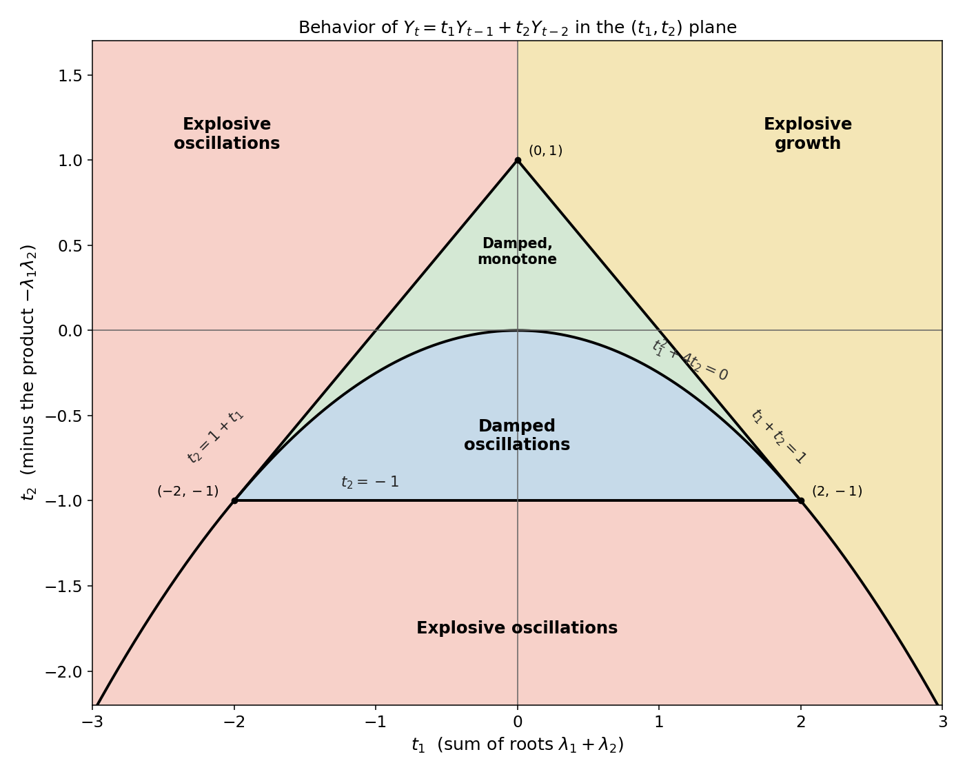
Fig. 1 Figure 1. Regions of the \((t_1, t_2)\) plane for \(Y_t = t_1 Y_{t-1} + t_2 Y_{t-2}\),
whose characteristic roots are \(\lambda = (t_1 \pm \sqrt{t_1^2 + 4 t_2})/2\). The downward
parabola \(t_1^2 + 4 t_2 = 0\) separates real roots (above) from complex-conjugate roots
(below). The stability triangle with edges \(t_1 + t_2 = 1\), \(t_2 = 1 + t_1\), and
\(t_2 = -1\) — vertices \((0,1)\) and \((\pm 2, -1)\) — encloses the parameter pairs for which
both roots are less than one in modulus. Inside the triangle the solution is damped:
oscillating below the parabola (complex roots), monotone above it (real roots). Outside
it the solution explodes, oscillating whenever the roots are complex or the dominant real
root is negative. Redrawn after W. Baumol, Economic Dynamics, 2nd ed., p. 221 (Macmillan,
1959). Generated by
code/ch09_fig1_stability_regions.py.#
A. An Example#
Maybe the most famous second-order difference equation in economics is the one associated with Samuelson’s multiplier accelerator model (see Samuelson, 1944). Samuelson posited the model
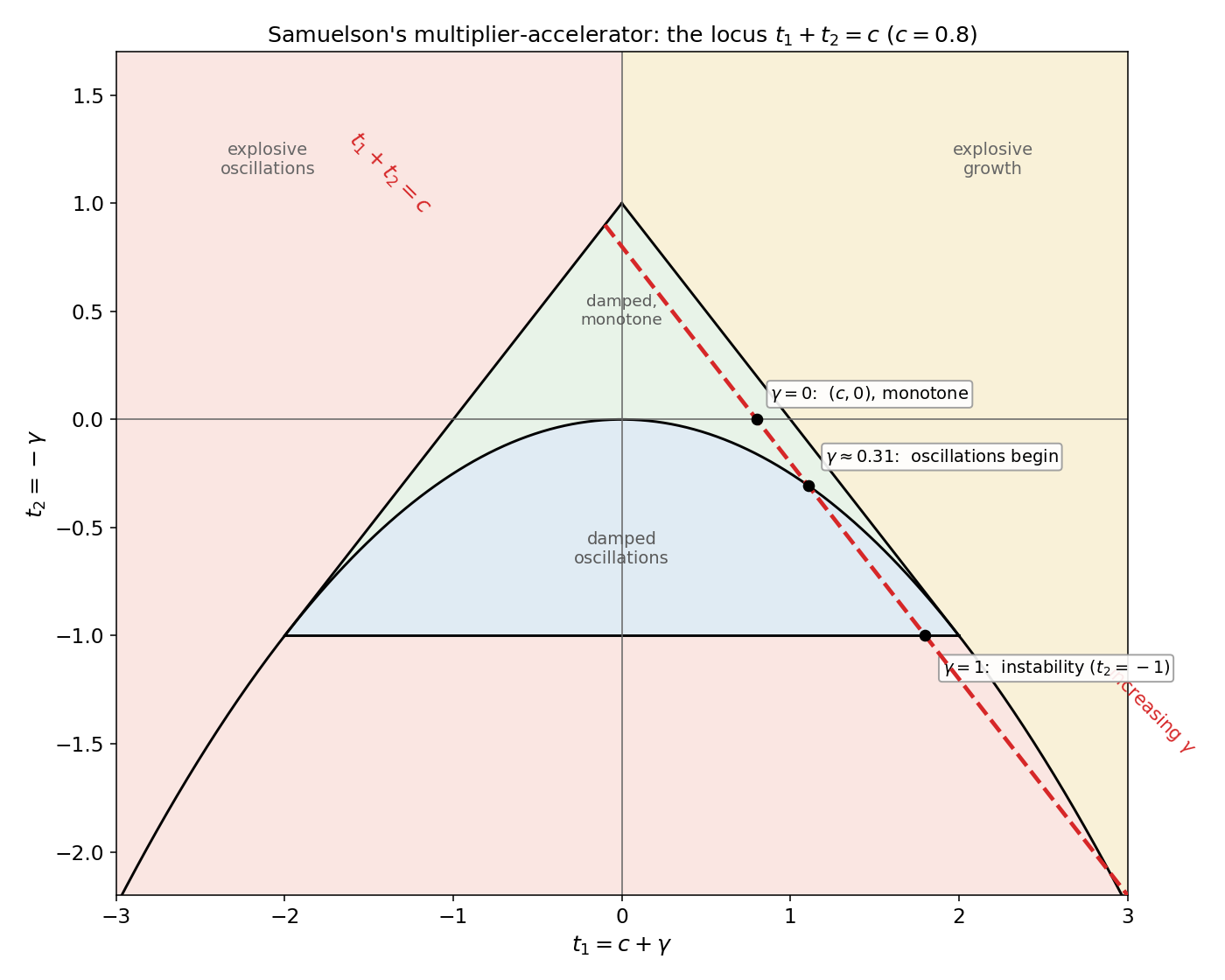
Fig. 2 Figure 2. Samuelson’s multiplier–accelerator model traces a straight path through the
plane of Figure 1. Because \(t_1 = c + \gamma\) and \(t_2 = -\gamma\), the parameter
point satisfies \(t_1 + t_2 = c\) for every value of the accelerator \(\gamma \geq 0\); as
\(\gamma\) rises the point slides down and to the right along this dashed line (here
\(c = 0.8\)), parallel to and just inside the stability edge \(t_1 + t_2 = 1\). Its crossings
with the region boundaries pick out the values of \(\gamma\) at which the model passes from
monotone convergence to damped oscillations (at the parabola, \(\gamma \approx 0.31\)) and
then from damped to explosive oscillations (at \(t_2 = -1\), \(\gamma = 1\)). Generated by
code/ch09_fig2_samuelson_locus.py.#
where \(C_t\) is consumption and \(I_t\) is investment. Substituting the first two equations into the third gives
or
where \(t_1 = c + \gamma\), \(t_2 = -\gamma\). Notice that \(t_1 + t_2 = c\). So increases in the parameter \(\gamma\) move the parameters \(t_1\) and \(t_2\) downward and to the right along the line
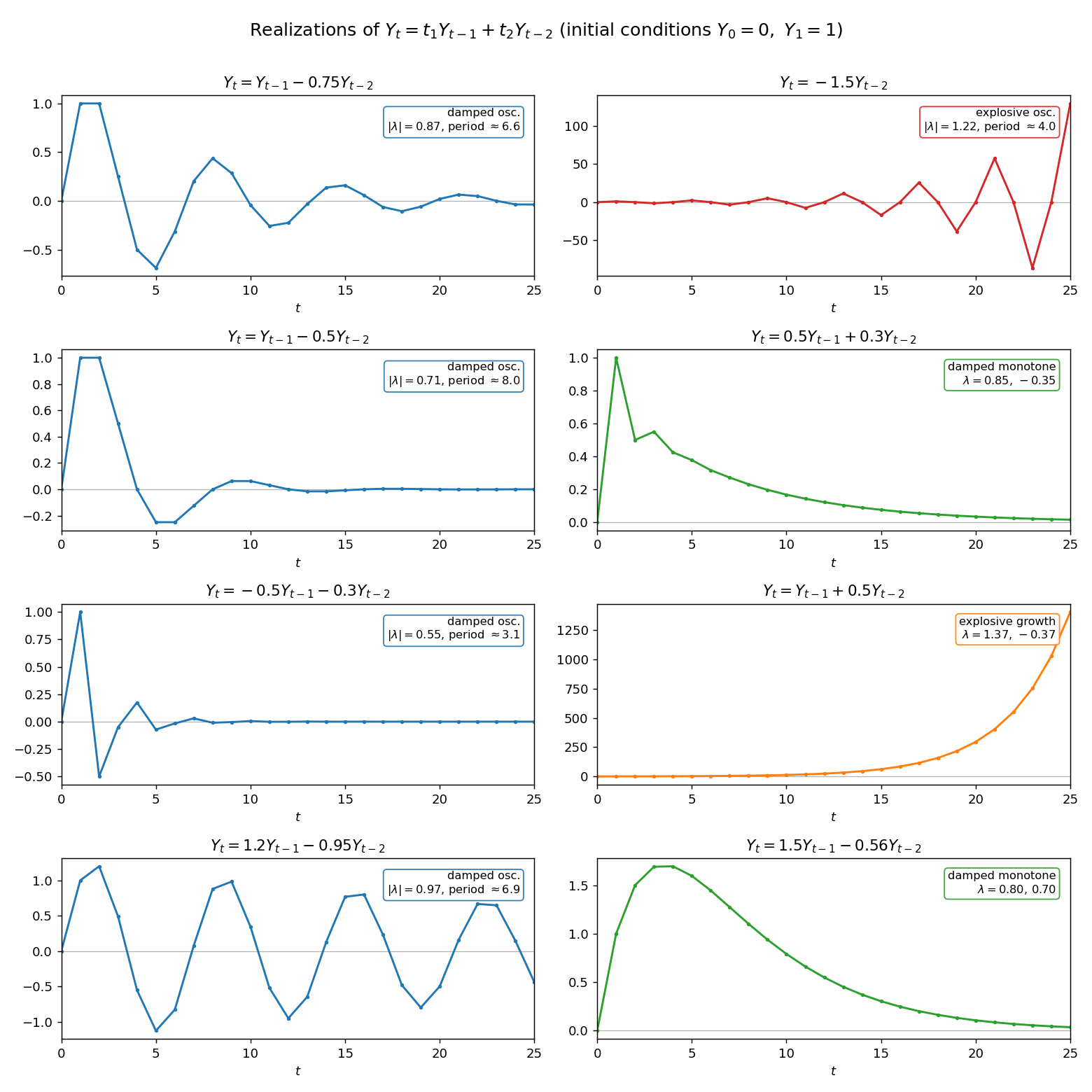
Fig. 3 Figure 3. Realizations of \(Y_t = t_1 Y_{t-1} + t_2 Y_{t-2}\) from the common initial
conditions \(Y_0 = 0,\ Y_1 = 1\), for eight parameter pairs that sweep the taxonomy of
Figure 1. Each panel reports the characteristic roots and the resulting behavior.
The qualitative pattern — damped or explosive, oscillatory or monotone — is set by where
\((t_1, t_2)\) sits in Figure 1, not by the initial conditions; the reader can check
each panel against its region. Note the very different vertical scales: the explosive cases
(\(Y_t = -1.5 Y_{t-2}\) and \(Y_t = Y_{t-1} + 0.5 Y_{t-2}\)) run off to large magnitudes, while
\(Y_t = 1.2 Y_{t-1} - 0.95 Y_{t-2}\), sitting just inside the unit circle, cycles for a long
time before decaying. Generated by
code/ch09_fig3_realizations.py.#
\(t_1 + t_2 = c\) in Figure 2. Using Figure 2, the values of \(c\) and \(\gamma\) compatible with damped oscillations, explosive oscillations, and so on, can easily be determined.
Figure 3 shows some realizations of second-order difference equations for various values of \(t_1\) and \(t_2\). In each case the values \(Y_0\) and \(Y_1\) were the two initial conditions which we specified arbitrarily. The reader can check that the behavior of these realizations matches that predicted by Figure 1.
3. Second-Order Difference Equations (Equal Roots)#
The preceding treatment assumed that \(\lambda_1 \neq \lambda_2\). (Notice that we divided by \(\lambda_1 - \lambda_2\) to obtain (21).) If \(\lambda_1 = \lambda_2\), then the polynomial we must study is
The lag distribution generated by the polynomial in (32) is called a second-order Pascal lag distribution. It is the lag operator product or “convolution” of two geometric lag distributions with the same decay parameter[5] \(\lambda\).
With the aid of (32) we can study the solution to difference equations of the form
The general solution is
where \(c_1\) and \(c_2\) are any real constants. To verify that (33) is the solution, operate on both sides by \((1 - \lambda L)^2\) and verify that \((1 - \lambda L)^2\{c_1\lambda^t + c_2 t\lambda^t\} = 0\) for any choices of \(c_1\) and \(c_2\). To get a particular solution, we require two side conditions on the path of \(Y_t\) to determine the two constants \(c_1\) and \(c_2\). For \(a\sum_{i=0}^{\infty}(1 + i)\lambda^i\) to be finite either \(|\lambda| < 1\) or \(a = 0\) must be satisfied.
Assume that \(a = 0\) and notice that (33) can be rewritten for \(t \geq 1\) as
The second sum can be written as
Therefore (34) becomes
where
As for our earlier cases, (35) displays the solution for \(t \geq 1\) as the sum of the distributed lag in \(X_1, X_2, \ldots, X_t\) and two initial conditions. If \(X_t = 0\) for \(t \geq 1\), the sequence \(Y_t\) will approach its stationary value of zero if \(|\lambda| < 1\). If \(|\lambda| > 1\), the sequence \(Y_t\) will diverge from the stationary point of zero unless \(\theta_0 = \eta_0 = 0\).
4. Nth-Order Difference Equations (Distinct Roots)#
Consider a rational polynomial with \(n\)th-order denominator:
We assume that the degree of the numerator polynomial is less than the degree of the denominator polynomial. The zeros of \(G(z) = 0\) are \(z_1 = 1/\lambda_1\), \(z_2 = 1/\lambda_2, \ldots, z_n = 1/\lambda_n\) since each of these values for \(z\) satisfies the equation
Suppose the \(n\) roots are distinct. Now the method of partial fractions enables us to express \(A(L)\) as
where \(A_1, A_2, \ldots, A_n\) are constants to be determined. To determine them, multiply both sides of the above equation by \((1 - \lambda_1 L) \cdots (1 - \lambda_n L)\) to get
Evaluating the above equation at \(L = 1/\lambda_1\), the first root of \(G(L) = 0\), gives
For the general term \(A_i\), we obtain
As an example, consider applying (36) to the second-order denominator polynomial
We have
Thus we obtain
which we earlier used on the way to deriving (21).
Suppose we have an \(n\)th-order difference equation
The general solution to (38) is obtained by “dividing”[6] by \((1 - \lambda_1 L) \cdots (1 - \lambda_n L)\) to obtain
where \(c_1, \ldots, c_n\) are any constants. That this is the solution can be verified by operating on both sides of the above equation with \((1 - \lambda_1 L) \cdots (1 - \lambda_n L)\). We now require \(n\) side conditions on the path of \(Y_t\) to determine the \(n\) constants \(c_1, \ldots, c_n\). We suppose that the \(\lambda_j\) are all distinct. Then application of (36) to the above equation gives
which shows that \(Y_t\) can be expressed as the weighted sum of \(n\) geometric distributed lags with decay coefficients \(\lambda_1, \lambda_2, \ldots, \lambda_n\).
Given \(n\) initial values of \(Y\), and assuming \(X_t = 0\) always, it is possible to start up difference equation (38) finitely far back in the past and to obtain a solution of the form
where \(\eta_1, \ldots, \eta_n\) are constants chosen to satisfy the \(n\) initial values. The above equation can be derived from (39) by applying calculations analogous to those applied above in the first- and second-order cases.
5. Nth-Order Difference Equations (N Equal Roots)#
Consider the \(n\)th-order difference equation
which has the solution
The polynomial \(1/(1 - \lambda L)^n\) is the one associated with an \(n\)th-order Pascal lag distribution, which is formed by multiplying (convolving) \(n\) geometric lag distributions with the same decay parameter \(\lambda\). We have already studied the second-order Pascal distribution. The binomial expansion with negative exponent is
Notice that \(n(n + 1) \cdots (n + i - 1) = (n + i - 1)!/(n - 1)!\) The coefficient on \(x^i\) in the above expansion is thus
Therefore, the expansion can be written
Consequently, for a lag-generating function[7] with \(n\) equal roots, we have
which agrees with our earlier formulas for the special cases \(n = 1\) and \(n = 2\).
To arrive at (41) in an alternative way, write
Differentiating with respect to \(\lambda L\) gives
which is (41) with \(n = 2\). Differentiating again with respect to \(\lambda L\) gives
or
which is (41) with \(n = 3\).
With the aid of (41), the solution to (40) can be written
6. An Example of a First-Order System#
Consider the following model studied by Cagan (1956). Let \(m_t\) be the log of the money supply, \(p_t\) the log of the price level and \(p_{t+1}^{\,\mathrm{e}}\) the log of the price expected to prevail at time \(t + 1\) given information available at time \(t\). The model is
which is a portfolio equilibrium condition. The demand for real balances varies inversely with expected inflation \(p_{t+1}^{\,\mathrm{e}} - p_t\). The variable \(m_t\) is exogenous.
Suppose first that
so that the public expects inflation next period to be the current rate of inflation, \(p_t - p_{t-1}\), multiplied by the constant \(\gamma\). Then (42) becomes
Using lag operators, this can be written as
or
The solution can be written
where \(c\) is a constant to be determined by, say, a given value of \(p\) at some time. The solution for \(p_t\) will be finite for the time path \(m_t = \bar{m}\) for all \(t\), provided that
The above inequality is in the spirit of the “stability condition” developed by Cagan in his paper. It is a condition that delivers a bounded \(p_t\) for all \(t \geq 0\) for \(\{m_t\}\) sequences that are bounded. Notice that
Thus, the long-run effect of a once-and-for-all jump in \(m\) is to drive \(p\) up by an equal amount (provided the above “stability condition” is met).
Returning to (42), let us abandon (43) and now assume perfect foresight:
Substituting (44) into (42) gives
Write this as
or
Notice that since \(\alpha < 0\), it follows that \((\alpha - 1)/\alpha > 1\). This fact is an invitation to solve (45) in the “forward” direction, i.e., to use (6). Dividing both sides of (45) by \((1 - ((\alpha - 1)/\alpha)L)\) gives
where \(c\) is any constant. Using (6), this becomes
Notice that since \(\alpha < 0\), \(0 < \alpha/(\alpha - 1) < 1\), so that the sum of the lag weights is finite. Equation (46) expresses the log of the current price as a moving sum of current and future values of the log of the money supply. Notice that
so that \(p\) is a weighted average of current and future values of \(m\). The solution for \(p_t\) given by (46) will be finite for all finite \(t\) if there is a constant \(K > 0\) and an \(x\), \(1 \leq x < (\alpha - 1)/\alpha\) such that \(|m_t| < Kx^t\) for all \(t\). This is a condition that the money supply not grow too fast. For the solution given by (46) to be bounded for money supply paths that are bounded, we would require that \(c = 0\). This amounts to an arbitrary terminal condition that rules out the occurrence of runaway inflations in the absence of runaway growth in the money supply.
7. An Example of a Second-Order System#
Consider the following model studied by Muth (1961). Let \(p_t\) be the price of a commodity at \(t\), \(C_t\) the demand for current consumption, \(I_t\) the stock of inventories of the commodity, \(Y_t\) the output of the commodity, and \(p_t^{\,\mathrm{e}}\) the price previously expected to prevail at time \(t\); \(\{X_t\}\) is a bounded sequence of real numbers that represents the effects of the weather on supply. The model is
Let us suppose that there is perfect foresight so that \(p_t^{\,\mathrm{e}} = p_t\) for all \(t\). Making this assumption and substituting the first three equations into the fourth gives
or
Dividing by \(\alpha\) gives
or
where \(\phi = ((\beta + \gamma)/\alpha) + 2 > 0\). Multiplying by \(L\) gives
We need to factor the polynomial \(1 - \phi L + L^2\) as
so that we require
The second equality establishes that \(\lambda_1 = 1/\lambda_2\), so that the two roots appear as a reciprocal pair. So we can write
where \(\lambda\) is chosen to satisfy \(\lambda + \lambda^{-1} = \phi\). So (47) can be written
Since \((\beta + \gamma)/\alpha > 0\), it follows that \(\phi = ((\beta + \gamma)/\alpha) + 2 > 2\). That implies that \(\lambda\) does not equal 1 since \(\lambda + \lambda^{-1} = \phi\). Notice that if \(\lambda > 1\), \(\lambda^{-1} < 1\). So one of our roots necessarily exceeds 1, the other necessarily is less than 1.
We divide both sides of (48) by \((1 - \lambda L)(1 - \lambda^{-1} L)\) to obtain
where \(c_1\) and \(c_2\) are any constants. Without loss of generality, suppose \(\lambda < 1\) and let \(\lambda_2 = 1/\lambda\). Use (6) and (21) to write the solution as
The solution (50) expresses \(p_t\) as a “two-sided” distributed lag of \(X\), i.e., as a weighted sum of past, present, and future values of \(X\). In this model the current price depends on the entire path of exogenous shock \(X\) over the entire past and the entire future. As usual, the constants \(c_1\) and \(c_2\) are determined from two side conditions on the path of \(p_t\). For example, if we were to impose the side conditions \(\lim_{t \to -\infty} |p_t| < \infty\), \(\lim_{t \to +\infty} |p_t| < \infty\), i.e., if we imposed boundedness on the \(p_t\) path for all bounded \(\{X_t\}\) sequences, then we would require \(c_1 = c_2 = 0\).
8. An Optimization Example: Solving a System of Euler Equations#
Thus far, our advice to solve stable roots backward and unstable roots forward has been to a certain extent arbitrary, being partly based on the desire to have solutions that are bounded. As it happens, when a linear difference equation emerges from a dynamic quadratic optimization problem, there are present additional necessary conditions for optimality which have precisely the effect of causing us to solve the stable root(s) backward and the unstable root(s) forward. We shall illustrate this for the case of a firm employing a single factor of production, labor, and facing a quadratic technology and quadratic costs of adjusting its labor force.
We consider a firm that at time \(t\) chooses employment to maximize its present value
\(n_{t-1}\) given. Here \(f_0\), \(f_1\), \(d > 0\) and the discount factor \(b\) obeys \(0 < b < 1\). Here \(w_{t+j}\) is the real wage faced by the firm at time \(t + j\), while \(n_{t+j}\) is the firm’s employment at \(t + j\). The firm faces a known sequence of \(\{a_{t+j}\}_{j=0}^{\infty}\), \(a_{t+j}\) being a shock to the marginal product of labor at time \(t + j\). We assume for all \(t\) that for some \(K > 0\), \(|w_t| < K(x)^t\), \(|a_t| < K(x)^t\), where \(1 \leq x < 1/\sqrt{b}\); sequences that satisfy these inequalities for some \(K > 0\) and \(1 \leq x < 1/\sqrt{b}\) will be termed of exponential order less than \(1/\sqrt{b}\). The firm faces costs of adjusting its labor force rapidly, which we model by deducting the term \(\frac{1}{2}d(n_{t+j} - n_{t+j-1})^2\) from real revenue each period. The firm faces known sequences \(\{w_{t+j}\}_{j=0}^{\infty}\) and \(\{a_{t+j}\}_{j=0}^{\infty}\) and is assumed to choose a sequence \(\{n_{t+j}\}_{j=0}^{\infty}\) to maximize \(v_t\).
In order to discover the appropriate solution to this problem it is convenient to consider the finite horizon problem: maximize
subject to \(n_{t-1}\) being given. This problem matches our infinite horizon problem when we drive \(T\) to infinity. If a sequence \(\{n_{t+j}\}_{j=0}^{T}\) is to maximize (52), it must satisfy the following system of first-order necessary conditions, which we derive by differentiating (52) with respect to \(n_t, n_{t+1}, \ldots, n_{t+T}\):
Equation (53) is a system of second-order linear difference equations known as the “Euler equations,” which we write as
or
To solve this second-order difference equation, we need two boundary conditions. One boundary condition is supplied by the historically given initial level of \(n_{t-1}\), and the other by the terminal condition (54). That terminal condition is known as the transversality condition and is a necessary condition for optimality. To get the terminal condition in the infinite horizon problem, it is appropriate to take
as the transversality condition. We obtain this condition by multiplying (54) by the terminal stock of employment \(n_{t+T}\), and taking the limit of the resulting equation as \(T \to \infty\). Sufficient conditions for the transversality condition (56) to hold are, first, that \(\{a_{t+j}\}\) and \(\{w_{t+j}\}\) be of exponential order less than \(1/\sqrt{b}\), and, second, that the solution for \(\{n_{t+j}\}\) be of exponential order less than \(1/\sqrt{b}\). Thus, suppose that \(\{w_t\}\), \(\{a_t\}\), and \(\{n_t\}\) are each of exponential order less than \(1/\sqrt{b}\). Then notice that
From the definition of a sequence of exponential order less than \(1/\sqrt{b}\), we have that \(0 < x\sqrt{b} < 1\). This condition implies that \(xb < \sqrt{b} < 1\). Therefore the limit as \(T \to \infty\) of the expression above equals zero. This proves that the conditions that \(\{a_t\}\), \(\{w_t\}\) and \(\{n_t\}\) are of exponential order less than \(1/\sqrt{b}\) are sufficient to imply that the transversality condition (56) is satisfied. The necessary conditions for optimality for the infinite horizon problem are then satisfied if we can find a solution to the difference equation
subject to the transversality condition (56) and the known initial value of \(n_{t-1}\).
To solve the difference equation, write it as
We seek a factorization
Equating powers of \(L\) gives
Thus we have that \(\lambda_1\) must satisfy
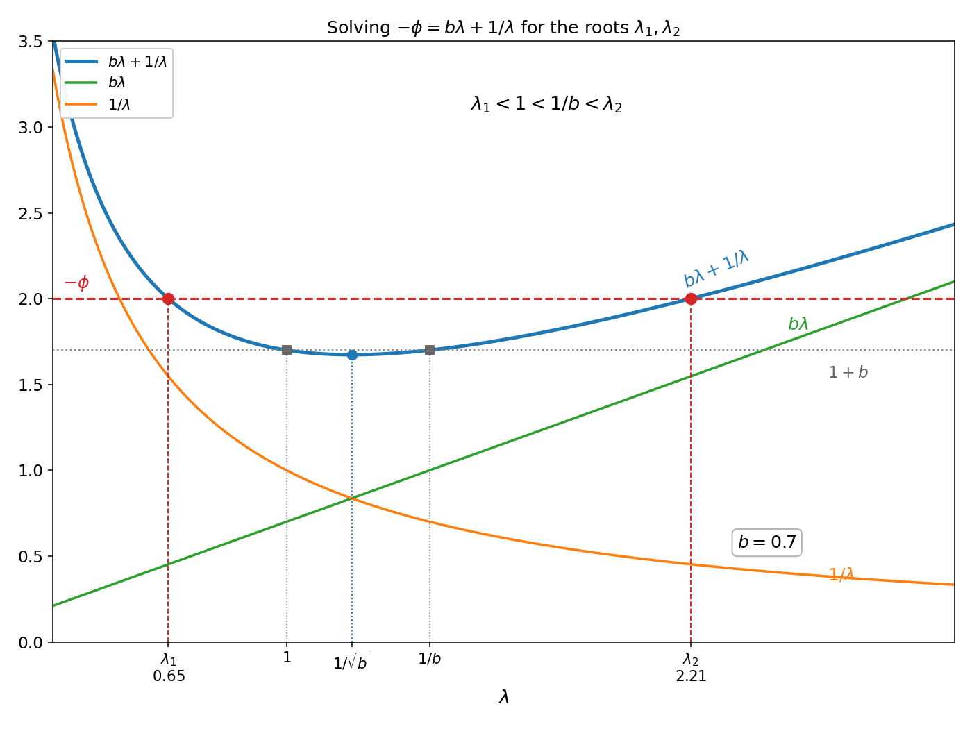
Fig. 4 Figure 4. Determining the factorization roots of the firm’s Euler equation. The roots
solve \(-\phi = b\lambda + 1/\lambda\), whose right-hand side (blue) is the sum of the line
\(b\lambda\) and the hyperbola \(1/\lambda\); it is U-shaped, with minimum value \(2\sqrt{b}\) at
\(\lambda = 1/\sqrt{b}\). A horizontal line at height \(-\phi\) cuts the curve at the two roots
\(\lambda_1 < \lambda_2\). Because \(-\phi = f_1/d + (1+b) > 1 + b\) whenever \(f_1 > 0\), and
because the line at height \(1+b\) meets the curve exactly at \(\lambda = 1\) and \(\lambda = 1/b\)
(the factorization of \(b\lambda^2 - (1+b)\lambda + 1\)), the two roots straddle both:
\(\lambda_1 < 1 < 1/b < \lambda_2\). The stable root \(\lambda_1 < 1\) builds the firm’s optimal
feedback rule; the unstable root \(\lambda_2 > 1/b\) is solved forward. Here \(b = 0.7\) and
\(-\phi = 2\). Generated by
code/ch09_fig4_root_determination.py.#
Figure 4 depicts the determination of \(\lambda_1\) and \(\lambda_2\). The function \(\lambda b + \lambda^{-1}\) attains a minimum at \(\lambda = \sqrt{1/b}\), attaining a value of \(2\sqrt{b}\) there. For \(0 < b < 1\), we have that \(1 + b \geq 2\sqrt{b}\) with equality at \(b = 1\), so that even with \(f_1 = 0\), in which case \(\phi = -(1+b)\), we have \(-\phi \geq 2\sqrt{b}\). This assures that with \(f_1 > 0\) the solutions for \(\lambda_1\) and \(\lambda_2\) as depicted in Figure 4 are real and distinct. Without loss of generality, let \(\lambda_1\) be the smaller root. Then notice that the preceding implies that \(\lambda_1 < 1/\sqrt{b} < \lambda_2\). By using Figure 4 we can establish that \(\lambda_1 < 1 < 1/b < \lambda_2\). From \(-\phi = ((f_1/d) + 1 + b)\), we have that \(-\phi > 1 + b\), since \(f_1/d > 0\). Now if \(-\phi\) were equal \(1 + b\), we would have \(\lambda_1\) and \(\lambda_2\) being determined from
or
so that \(\lambda_1 = 1\), \(\lambda_2 = 1/b\). Since \(-\phi > 1 + b\), inspection of Figure 4 shows that unity must be an upper bound for \(\lambda_1\) and \(1/b\) a lower bound for \(\lambda_2\).[8]
Having achieved this factorization, we write the difference equation as
To satisfy the transversality condition, operate on both sides of this equation with the “forward” inverse of \(1 - \lambda_2 L\) to get
where \(c\) is a constant. However, since \(\lambda_2 > 1/b > 1/\sqrt{b}\), we must set \(c = 0\) in order to satisfy the transversality condition, for otherwise \(\{n_{t+j}\}\) would fail to be of exponential order less than \(1/\sqrt{b}\). Setting \(c = 0\) and observing that \(1/\lambda_2 = b\lambda_1\), we have
This is a demand schedule for employment that expresses current employment as a function of once-lagged employment and current and all future values of the real wage and the shock to productivity. Since \(\lambda_2 > 1/b\), we have that \(1/\lambda_2 < b\), so that the infinite weighted sum on the right-hand side of (57) converges for \(\{a_{t+j}\}\) and \(\{w_{t+j}\}\) sequences that are of exponential order of less than \(1/b\). We have assumed the stronger condition that \(\{a_t\}\), \(\{w_t\}\) are sequences of exponential order less than \(1/\sqrt{b}\), so that the infinite weighted sum on the right side of (57) converges.
It remains to show that (57) holds for \(j = -1\) as well. To show this, take the solution (57) for \(j = 0\) and use it to eliminate \(n_{t+1}\) from the Euler equation (55) for \(j = 0\), thereby obtaining
where \(z_t \equiv d^{-1}(w_t - a_t - f_0)\). Since \(\lambda_1 + \lambda_2 = -\phi/b\) and \(b\lambda_1 = \lambda_2^{-1}\), we can rearrange the above equation to read
which asserts that (57) holds for \(j = -1\). Thus, (57) gives the firm’s optimal plan for setting \(n_{t+j+1}\) for \(j = -1, 0, 1, \ldots\).
We have in effect imposed the transversality condition first by using the “unstable” root \(\lambda_2\) to solve in the forward direction and second by setting \(c\lambda_2^t = 0\) in (57). To see this, write (57) as
where
Since \(\{w_{t+j}\}\) and \(\{a_{t+j}\}\) are of exponential order less than \(1/\sqrt{b}\), it follows[9] that the sequence \(\{\varepsilon_{t+j+1}\}\) is of exponential order less than \(1/\sqrt{b}\) and is finite for finite \(t + j\). The solution of the difference equation (57) with \(n_{t-1}\) given is
This is the unique solution to the Euler equation that satisfies the initial condition and the transversality condition (56). It is straightforward to verify that both the initial condition and the transversality condition are satisfied by this solution, the latter condition being satisfied by virtue of the exponential order being less than \(1/\sqrt{b}\) for the \(\{\varepsilon_{t+j}\}\) sequence and the fact that \(|\lambda_1| < 1\). For notice that
which proves that \(\sum_{i=0}^{j+1} \lambda_1^i \varepsilon_{t+j+1-i}\) is of exponential order less than \(1/\sqrt{b}\). It follows that (59) implies that \(n_{t+j}\) is of exponential order less than \(1/\sqrt{b}\), and therefore that the transversality condition (56) is satisfied.
It should be emphasized that the transversality condition compels us to solve the unstable root forward. If we had solved the unstable root \(\lambda_2\) “backward,” then eventually the solution for \(n_{t+j+1}\) would come to be dominated by terms of exponential order \(\lambda_2\). Since \(\lambda_2 > 1/\sqrt{b}\), that solution would violate the transversality condition (56).
In conclusion, the solution of our infinite horizon maximum problem is for the firm to set its employment according to the demand schedule or decision rule
for \(j = -1, 0, 1, 2, \ldots\).
9. A More General Univariate Optimization Problem#
The problem of the preceding section is a special case of a more general quadratic optimization problem, one version of which follows. We define the polynomial in the lag operator,
where \(d_0 \neq 0\), \(d_m \neq 0\). We assume that \(g_t\) is a sequence of exponential order less than \(1/\sqrt{b}\), where \(0 < b < 1\). Then the problem is to choose a sequence \(\{y_t, t \geq 0\}\) to maximize
where \(h > 0\), subject to \(y_{-1}, y_{-2}, \ldots, y_{-m}\) given. The problem of Section 8 is a version of problem (61) with \(g_t = (f_0 + a_t - w_t)\), \(m = 1\), \(y_t = n_t\), and \(d(L) = \sqrt{d}(1 - L)\), \(h = f_1\).
The Euler equation for this problem is
We invite the reader to verify that this is the Euler equation by differentiating (61) with respect to \(y_t\) and rearranging. Note that (55) is a special case of (62) with \(d(L) = (1 - L)\sqrt{d}\), \(h = f_1\), \(g_t = (f_0 + a_t - w_t)\).
In addition to the Euler equation (62), the necessary and sufficient conditions for maximization of (61) are completed by the condition
Inspection of (61) reveals that any \(\{y_t\}\) path that violates (63), even if it satisfies the Euler equation, gives a very bad outcome for the criterion function. Imposing conditions (63) is equivalent to imposing transversality conditions. Transversality conditions could be derived as in Section 8, by differentiating a finite \(T\) version of (61) with respect to \(y_T, \ldots, y_{T-m+1}\), multiplying the resulting \(m\) expressions by \(y_T, \ldots, y_{T-m+1}\), respectively, and setting the limits as \(T \to \infty\) to zero. As do the transversality conditions, (63) forces the solution \(\{y_t\}\) to be of exponential order less than \(1/\sqrt{b}\).
We briefly describe how (62) is solved subject to (63). We first note a simple but important feature of the characteristic polynomial \(h + d(bL^{-1}) d(L)\) that appears in (62). This polynomial evaluated at any value \(z_0\) equals the polynomial evaluated at \(b z_0^{-1}\). In particular, if \(z_0\) is a zero of this polynomial, then so is \(b z_0^{-1}\). To prove this, suppose that \(z_0\) is a zero, which means setting \(L = z_0\) gives \(h + d(b z_0^{-1}) d(z_0) = 0\). The claim is that this implies that setting \(L = b z_0^{-1}\) will also set the polynomial to zero. Making this substitution gives \(h + d(z_0) d(b z_0^{-1})\), which equals the characteristic polynomial evaluated at \(z_0\), which equals zero by assumption. Thus, the zeros of the characteristic polynomial of the Euler equation come in pairs of the form \(z_k, b z_k^{-1}\), \(k = 1, \ldots, m\).
Let us assume that the zeros of the characteristic polynomial are distinct. (The reader can apply the methods of Section 5 to analyze the case of repeated zeros, if this becomes necessary.) There are \(2m\) zeros of the polynomial \(h + d(b z^{-1}) d(z)\). Denote these zeros \(z_1, z_2, \ldots, z_{2m}\). Without loss of generality, let the zeros be arranged in descending order according to their absolute value. Then we have that the zeros are ordered as \(|z_1| \geq |z_2| \geq \cdots \geq |z_m| > |b z_m^{-1}| \geq |b z_{m-1}^{-1}| \geq \cdots \geq |b z_1^{-1}|\). (The weak inequalities leave open the possibility that there are complex roots.) Let us define \(\lambda_k = 1/z_k\), \(k = 1, \ldots, m\). Notice that the above ordering, and in particular \(|z_m| > |b z_m^{-1}|\), implies that \(|\lambda_k| < 1/\sqrt{b}\) for \(k = 1, \ldots, m\). Then it is possible to factor the characteristic polynomial of the Euler equation as
where
and where \(\lambda_0\) is a constant that is uniquely determined by \(h\) and \(d(L)\).
Since \(|\lambda_k| < 1/\sqrt{b}\) for \(k = 1, \ldots, m\), (64)–(65) imply that \(h + d(bL^{-1}) d(L)\) has been factored into \(c(bL^{-1}) c(L)\), where the zeros of \(c(z)\) exceed \(\sqrt{b}\) in modulus, (from (65) the zeros of \(c(z)\) are the \(1/\lambda_k\)’s) and where the zeros of \(c(bz^{-1})\) are less than \(\sqrt{b}\) in modulus.
Using factorization (64), the Euler equation (62) can be represented as
The unique solution of the Euler equation that satisfies (63) is given by
or
A partial fraction representation of \(c_0 c(bL^{-1})^{-1}\) is given by
where
Using (69), solution (68) can be represented as
or
Since \(|\lambda_k| < 1/\sqrt{b}\), \(|b\lambda_k| < \sqrt{b}\). This condition, together with our having assumed that \(\{g_t\}\) is of exponential order less than \(1/\sqrt{b}\) guarantees that the right hand side converges, and that as a function of \(t\) it is itself of exponential order less than \(1/\sqrt{b}\). It follows that the solution (72) starting from the given starting values \(y_{-1}, \ldots, y_{-m}\) satisfies condition (63) and is therefore optimal.
We close this section with a remark on terminology. Consider solution (68), \(c(L) y_t = c(bL^{-1})^{-1} g_t\). In the control literature, \(c(L) y_t\) is called the “feedback part” of the solution for \(y\), while \(c(bL^{-1})^{-1} g_t\) is called the “feedforward part.”
10. Introduction to Multivariate Dynamic Optimization#
We now briefly describe a multivariate generalization of the problem of Section 9, and its solution. This section is a brief introduction to ideas described more fully in Hansen and Sargent [1981]. We define the matrix polynomial in the lag operator
where \(D_j\) is an \((n \times n)\) matrix. We let \(\{G_t\}\) be a sequence of \((n \times 1)\) vectors, each component of which is a sequence of exponential order less than \(1/\sqrt{b}\). We let \(H\) be an \((n \times n)\) positive definite matrix. Finally, we let \(\{Y_t\}\) be a sequence of \((n \times 1)\) vectors of variables that are to be chosen for \(t \geq 0\), with given initial values \(Y_{-1}, Y_{-2}, \ldots, Y_{-m}\). The problem we are interested in is to choose \(\{Y_t, t \geq 0\}\) to maximize
given \(\{G_t, t \geq 0\}\) and \(Y_{-1}, \ldots, Y_{-m}\). In (74), the prime \((')\) denotes matrix transposition.
Necessary and sufficient conditions for a maximum of (74) are
and the Euler equations
That the Euler equations assume the form (76) can be proved using the method of Sections 8 and 9, namely by differentiating (74) with respect to \(Y_t\), equating the result to a vector of zeros, and rearranging. Condition (75) is the correct generalization of (63), and is justified by similar reasoning.
The related-pairs property of the zeros of the characteristic polynomial of the Euler equation that held in the univariate case generalizes as follows.
If \(z_0\) is a zero of \(\det\{H + D(bz^{-1})'D(z)\}\) then so is \(bz_0^{-1}\). Here “det” denotes the determinant of a matrix. The appropriate matrix analogue of the scalar polynomial factorization (64) is a matrix polynomial factorization \(C(bL^{-1})'C(L)\), where the zeros of \(\det C(z)\) exceed \(\sqrt{b}\) in absolute value, while those of \(\det C(bz^{-1})\) are less than \(\sqrt{b}\) in absolute value. By a theorem on matrix polynomials of the form that appears in (76), there always exists a matrix factorization
where
and where the zeros of \(\det C(z)\) exceed \(\sqrt{b}\) in absolute value.
The solution of (76) satisfying (75) is then given by
By the above mentioned property of the location of the zeros of \(\det C(bz^{-1})\), we can represent \(\det C(bL^{-1})'\), as
where \(|\lambda_j| < 1/\sqrt{b}\), \(j = 1, \ldots, k\), where \(k = mn\), and where we have assumed distinct zeros of \(\det C(bz^{-1})\). Using a matrix version of partial fractions, \(C(bL^{-1})'^{-1}\) can be represented as
where
Note that each \(A_h\) is an \((n \times n)\) matrix. Using (80), (79) can be represented
Representation (82) is the vector generalization of (72).
Note in (79) a sort of symmetry in form between the “feedback part” \(C(L)Y_t\) and the “feedforward part” \(C(bL^{-1})'^{-1}G_t\) that generalizes a similar symmetry that we observed in the univariate problems.
A key step in solving problems of this sort is achieving the matrix factorization (77). Hansen and Sargent (1981) describe several methods for accomplishing this.
Example (ii): A Dynamic Nash Equilibrium[10]#
We consider a duopoly in an industry producing a single good. Demand is governed by a linear demand schedule,
where \(q_{it}\) is output of firm \(i\) at \(t\), \(p_t\) is the price of output at \(t\), and \(u_t\) is a given sequence of disturbances to demand of exponential order less than \(1/\sqrt{b}\). Firm \(i\) maximizes
where \(d_i(L) = d_{i0} + \cdots + d_{im}L^m\), and where \(s_{it}\) is a sequence of shocks to costs of production of firm \(i\), assumed to be a known sequence of exponential order less than \(1/\sqrt{b}\). Here \([d_i(L)q_{it}]^2\) stands for costs of adjusting production rapidly. The maximization of (87) by \(i\) takes \(\{s_{it}\}\), \(\{u_t\}\), and \(\{q_{jt}, j \neq i\}\) given for \(t \geq 0\), and \(q_{it}\) given for \(\{t = -m, \ldots, -1\}\), \(i = 1, 2\). In particular, firm \(i\) is supposed to regard firm \(j\)’s output sequence as given and beyond its influence.
Substituting (86) into (87) gives
The Euler equations for this problem for firms 1 and 2 are
We define a Nash equilibrium in the space of sequences of quantities \(q_{1t}\), \(q_{2t}\) as a pair of sequences for \(q_{1t}\), \(q_{2t}\)[11] that solve the interrelated Euler equations (89) and satisfy the boundary conditions
Equivalently, the Nash equilibrium is the pair of \((q_{1t}, q_{2t})\) sequences that satisfies the following conditions:
(i) Firm \(i\)’s quantity sequence maximizes its present value (87), given firm \(j\)’s sequence, for \((i, j) = (1, 2)\) and \((2, 1)\).
(ii) The output market clears, in the sense that (86) holds for all \(t\).
Equation (89) is evidently in the form of a vector Euler equation in \((q_{1t}, q_{2t})\). The matrix polynomial on the left side of (89) can be factored into the form
\(C(bL^{-1})'C(L)\), where \(C(L)\) is a \((2 \times 2)\) matrix polynomial with the zeros of \(\det C(z)\) exceeding \(\sqrt{b}\) in absolute value. Then the Nash equilibrium can be represented
where
Note that the vector Euler equation (89) was discovered by our having solved an interrelated pair of univariate dynamic optimization problems. The resulting system of Euler equations (89) can itself be viewed as solving some vector optimization problem, since the matrix characteristic polynomial is expressible in the form \(H + D(bL^{-1})'D(L)\). To seek the vector dynamic optimization problem that is implicitly solved by (89) is to pose a version of an “inverse optimal control problem:” given a system of difference equations, attempt to synthesize an optimum problem for which they are necessary conditions.[12][13]
11. Another Example: Learning by Doing#
The following example is interesting from both a substantive and a technical point of view. From a technical point of view, the example will introduce a control problem in which a rational characteristic polynomial must be factored in order to solve the Euler equation.
We consider a monopolist who faces the linear law of demand
where \(p_t\) is price, \(Q_t\) is output, and \(u_t\) is a known sequence of shocks to demand, assumed to be of exponential order less than \(1/\sqrt{b}\). The monopolist’s total costs at \(t\) are given by
where \(s_t\) is a known sequence of shocks to marginal cost, assumed to be of exponential order less than \(1/\sqrt{b}\), where \(h(L) = \sum_{j=0}^{\infty} h_j L^j\). As an example of the sort of \(h(L)\) that we have in mind, we shall later consider the special case \(h(L) = 1/(1 - \rho L)\) where \(\rho < 1\) but where \(\rho\) is close to one. Then (92) captures the notion that marginal costs of current output fall with cumulated past output. This is one version of a “learning-by-doing” cost structure.
The firm maximizes
The firm chooses a sequence \(\{Q_t\}_{t=0}^{\infty}\) to maximize (93), taking as given \(Q_t\) for \(t < 0\) and the sequences \(\{u_t\}_{t=0}^{\infty}\), \(\{s_t\}_{t=0}^{\infty}\). By using the preceding method, the Euler equation for the firm’s problem is found to be, after some rearrangement,
For convenience, set \(c_1 = 0\). The boundary condition is
We shall now consider the special case of the model that emerges when we set \(h(L) = 1/(1 - \rho L)\), \(0 < \rho < 1\). In this case, the characteristic polynomial on the left side of the Euler equation (94) becomes the rational polynomial
where \(k \equiv (A_1 + c_2)\). To solve the Euler equation (94) subject to boundary condition (95), the first step is to express the characteristic polynomial in terms of a common denominator, which gives
Notice that the denominator is already factored, and that the zeros of the numerator come in the familiar pair \((z_0, bz_0^{-1})\). Our next step on the way to solving our problem is to factor the numerator. Note that the numerator is proportional to
where \(1/\alpha\) is the zero of the characteristic polynomial that exceeds \(1/\sqrt{b}\). Equating powers of \(L\), as in section 8, shows that \(\alpha\) must solve
We assume that the parameter \(k \equiv A_1 + c_2\), \(c_4\), \(\rho\), \(b\) are such that the right side exceeds \(2\sqrt{b}\) in absolute value. This guarantees the existence of a real number \(\alpha\) that solves (98). Note that for \(\rho = b = 1\), the above equation has the solution \(\alpha = 1/\alpha = 1\). By continuity of the solution in the arguments on the right hand side, for values of \(\rho\) and \(b\) sufficiently close to 1, \(\alpha\) will be close to one.
Using (96) and (97), the Euler equation can be expressed
The solution of the Euler equation (99) that satisfies boundary condition (95) can be expressed in “feedback-feedforward” form
Unless \(\alpha = \rho\), \(Q_t\) feeds back on an infinite number of its own past values, reflecting the dynamics of the firm’s optimally coping with the learning-by-doing cost structure. In general, \(\rho \neq \alpha\). However, in the special limiting case \(\rho = b = 1\), it can be verified that \(\rho = \alpha\). In this special case, (100) collapses to the static decision rule
despite the presence of the learning-by-doing cost structure.
12. A Consumption Example#
We begin with a technical remark. Suppose that we wish to differentiate with respect to \(x_t\) the expression
where \(a(L) = \sum_{j=-\infty}^{\infty} a_j L^j\), \(d(L) = \sum_{j=-\infty}^{\infty} d_j L^j\). We invite the reader to verify that
We shall apply this formula in studying an optimal consumption problem.
A consumer is assumed to maximize
subject to
and
Here \(c_t\) is consumption, \(y_t\) is labor income, \(A_t\) is nonhuman assets available at the beginning of period \(t\), and \(R\) is the gross rate of return on nonhuman assets. We assume that \(0 > B > -\infty\), so that (104) requires that assets be uniformly bounded from below. This condition rules out a strategy of consuming large amounts and financing it by borrowing along an increasing and unbounded path.
Use (103) to express \(c_t\) as
Substituting (106) into (102) gives the criterion
which is to be maximized by selecting a sequence for \(A_t\), subject to the boundary conditions (104) and (105). Repeatedly applying formula (101), we find the Euler equation
The zeros of the characteristic polynomial in \(A_t\) are at \(L = R^{-1} < 1\) and \(L = Rb\). In order to satisfy the boundary conditions (104) and (105), the polynomial \((R^{-1}L^{-1} - 1)\) must be solved forwards, and the polynomial \((R^{-1}b^{-1}L - 1)\) solved backwards. Dividing (108) by \((R^{-1}L^{-1} - 1)\) gives
or
Subtracting (109) from (103) lagged one period, namely,
gives
or
Writing out the polynomial in \(L\) explicitly and shifting forward one period gives
This is a certainty version of the permanent income theory of consumption. According to (111), consumption is a linear function of wealth, defined as the sum of nonhuman wealth \(A_t\) and the discounted present value of labor income, \(\sum_{j=0}^{\infty} R^{-j}y_{t+j}\). In the special case that \(bR = 1\), (111) collapses to
It is also true that when \(Rb = 1\), (111) and (103) imply that \(c_t = c_0\) for all \(t\), so that the model implies complete consumption smoothing. To convince oneself of this, the reader is invited to verify that the Euler equation of this model can be represented as
Robert Hall [1978] pursued the empirical implications of a stochastic version of such an Euler equation. In Chapter XII of Macroeconomic Theory, we study this consumption example further.
13. Nonanticipative Representations and Lucas’s Critique#
We return to a version of the difference equation associated with Cagan’s model of hyperinflation, which we studied in Section 6 above. In particular, we have
where \(\{x_t\}\) is a sequence of exponential order less than \(1/\lambda\). The unique bounded solution of this equation is given by
This equation represents the solution for \(y_t\) in terms of an infinite number of future values of the “forcing variable” \(x_t\). In practice, one often prefers a “nonanticipative” representation of a solution, in which \(y_t\) is expressed as a solution only of \(x\)’s dated \(t\) and earlier. We now briefly show how representation (112) can be converted to an alternative representation expressing \(y_t\) as such a function of current and past \(x\)’s only. Given (112), such a representation in terms of current and past \(x\)’s can be attained by positing a specific difference equation for \(\{x_t\}\) itself, using this difference equation to express \(x_{t+j}\) for \(j \geq 1\) as functions of \(\{x_t, x_{t-1}, \ldots\}\), and then using these functions to eliminate \(x_{t+j}\) for \(j \geq 1\) from (112). The parameters of the representation for \(y_t\) as a function of current and past \(x\)’s will depend on the parameters of the difference equation for \(x_t\). This is so because the representation expressing \(y_t\) as a function of \(\{x_t, x_{t-1}, \ldots\}\) incorporates the solution of the difference equation expressing \(x_{t+j}\), \(j \geq 1\), in terms of \(\{x_t, x_{t-1}, x_{t-2}, \ldots\}\). For example, suppose that \(x_t\) is governed by the difference equation
Then we have that
Substituting this into (112) gives
which is an expression for \(y_t\) in terms of \(x_t\) in which the parameter \(\rho\) of the difference equation for \(x_t\) appears.
More generally, assume that \(x_t\) is governed by the difference equation
where \(a(L) = 1 - a_1 L - a_2 L^2 - \cdots - a_r L^r\) and where the zeros of \(a(z)\) exceed \(1/\lambda\) in absolute value. Then Hansen and Sargent (1980) show that the solution of (112) can be represented as
(We shall show how to derive this formula in §20.) Equation (115) is evidently a generalization of (113). That is, (113) is (115) for the case \(r = 1\), \(a_0 = 1\), \(a_1 = \rho\).
Equations (114) and (115) display a hallmark of economic models incorporating foresight as in (112), namely the presence of cross-equation restrictions between, on the one hand, the parameters of the process \(\{x_t\}\) of the forcing variables, and, on the other hand, the solution for \(y_t\) in terms of \(\{x_t, x_{t-1}, \ldots\}\). This characteristic of models with foresight means that it will not be possible to find a representation expressing \(y_t\) as a function of \(\{x_t, x_{t-1}, \ldots\}\) that is independent of the law of motion (difference equation) governing the forcing process \(\{x_t\}\). Alterations in the law of motion for \(x_t\) will alter the function describing the dependence of \(y_t\) on current and past \(x\)’s.
The presence of such cross-equation restrictions in models with foresight is the source of Robert E. Lucas’s (1976) criticism of some econometric policy evaluation procedures of the past. Lucas criticized methods that took representations of a variable like \(y_t\) as a function of \(\{x_t, x_{t-1}, \ldots\}\) and treated them as being invariant with respect to alterations in the difference equation generating the \(\{x_t\}\) sequence.
Exercises#
Exercise 1
Verify that the presence of both lagged employment and future values of \(w_t\) and \(a_t\) on the right-hand side of the employment decision rule (57) (demand schedule) depends on having the adjustment cost parameter \(d\) strictly positive. (Set \(d = 0\) and rework the firm’s optimum problem.)
Solution to Exercise 1
Set \(d=0\) in the present value (51). The adjustment-cost term \(\frac{d}{2}(n_{t+j}-n_{t+j-1})^2\) vanishes, so nothing links employment across periods and the problem separates date by date:
The first-order condition \(f_0 + a_{t+j} - w_{t+j} - f_1 n_{t+j} = 0\) gives
which depends only on the current shock and wage — there is no lagged employment and no dependence on future \(w\) or \(a\). Both of those features of the decision rule (57) are therefore artifacts of \(d>0\). The limit confirms it: the stable root solves \(\lambda_1 b + \lambda_1^{-1} = f_1/d + 1 + b\), so as \(d\to 0\) the right side \(\to\infty\), giving \(\lambda_1 \approx d/f_1 \to 0\) and \(\lambda_2 = 1/(b\lambda_1)\to\infty\). In (57) the feedback coefficient \(\lambda_1\to 0\) and the forward weights \(\lambda_2^{-i}\to 0\) for \(i\ge1\), leaving only \(-(\lambda_1/d)(w_{t+j+1}-a_{t+j+1}-f_0)\to (f_0+a_{t+j+1}-w_{t+j+1})/f_1\) — the static rule again.
Exercise 2
Determine the effect of an increase in \(d\) on the speed of adjustment parameters \(\lambda_1\) and \(\lambda_2\). Does a firm facing a small \(d\) adjust its labor force more or less quickly in response to current conditions than a firm facing a larger value of \(d\)? (Hint: use Figure 4.)
Solution to Exercise 2
The stable root satisfies \(\lambda_1 b + \lambda_1^{-1} = f_1/d + (1+b) = -\phi\) (see (55) and Figure 4). On the branch \(0<\lambda_1<1/\sqrt b\) the function \(\lambda b + \lambda^{-1}\) is decreasing, so a smaller value of \(-\phi\) corresponds to a larger \(\lambda_1\).
Increasing \(d\) lowers \(f_1/d\), hence lowers \(-\phi\) toward its floor \(1+b\); by that monotonicity it raises \(\lambda_1\) toward \(1\) (and lowers \(\lambda_2\) toward \(1/b\)). In the feedback rule \(n_{t+j+1}=\lambda_1 n_{t+j}+\cdots\) the number \(\lambda_1\) is the coefficient on lagged employment, so the speed of adjustment toward the target is \(1-\lambda_1\).
Therefore a firm facing a larger \(d\) has \(\lambda_1\) closer to \(1\) and adjusts more slowly, while a firm facing a small \(d\) has \(\lambda_1\) near \(0\) and adjusts quickly (in the limit \(d\to0\), \(\lambda_1\to0\) and it jumps straight to the frictionless target of Exercise 1). Larger adjustment costs make it optimal to spread employment changes over more periods.
Exercise 3
(A Keynesian investment schedule) A firm chooses a sequence of capital \(\{k_{t+j}\}_{j=0}^{\infty}\) to maximize
given \(k_{t-1} > 0\), where \(a_0, a_1, d > 0\) and where \(\{J_{t+j}\}_{j=0}^{\infty}\) is a known sequence of the price of capital relative to the price of the firm’s output. The sequence \(\{J_{t+j}\}\) is of exponential order less than \(1/b\), where \(0 < b < 1\) is the discount factor (the reciprocal of one plus the real rate of interest).
A. Derive the Euler equations and the transversality condition.
B. Show that the optimum decision rule of the firm is of the form
where \(0 < \lambda_1 < 1 < \lambda_2\), and \(c_0\) and \(c_1\) are constants. Find \(c_0\) and \(c_1\); show how to find \(\lambda_1\) and \(\lambda_2\); and prove that the \(\lambda\)’s obey the inequalities just stated.
Solution to Exercise 3
A. \(k_{t+j}\) enters the date-\((t+j)\) term directly and the date-\((t+j+1)\) adjustment terms through \(k_{t+j+1}-k_{t+j}\). Differentiating \(v_t\),
which rearranges to the Euler equation
with transversality condition \(\lim_{T\to\infty} b^{T}\big[a_0 - a_1 k_{t+T} - J_{t+T} - d(k_{t+T}-k_{t+T-1})\big]k_{t+T}=0\), satisfied when \(\{J\}\) and \(\{k\}\) are of exponential order less than \(1/\sqrt b\).
B. Factor \(b(1-\lambda_1 L)(1-\lambda_2 L)k_{t+j+1}=\tfrac1d(J_{t+j}-bJ_{t+j+1}-a_0)\) with \(\lambda_1\lambda_2=1/b\) and \(\lambda_1 b + \lambda_1^{-1} = a_1/d + 1 + b\). Since \(a_1/d>0\), the right side exceeds \(1+b\); the line at height \(1+b\) meets \(b\lambda+\lambda^{-1}\) exactly at \(\lambda=1\) and \(\lambda=1/b\) (as in Figure 4), so the roots straddle them: \(0<\lambda_1<1<1/b<\lambda_2\). Solving the stable root backward and the unstable root forward (dropping the \(\lambda_2^t\) term to meet transversality, and using \(1/\lambda_2=b\lambda_1\)),
The constant \(c_0\) places the rule’s rest point at the frictionless target \(\bar k=(a_0-(1-b)\bar J)/a_1\), where marginal product \(a_0-a_1k\) equals the user cost of capital.
Exercise 4
(Keynesian stabilization policy) The reduced form for GNP (\(Y\)) is
where \(g\) is government purchases and \(S_t\) is exports, an exogenous variable outside the government’s control. The sequence of exports \(\{S_t\}_{t=0}^{\infty}\) is of exponential order less than \(1/b\) where \(0 < b < 1\). Suppose that the government sets \(g_t\) to minimize the loss function
where \(\{Y_t^*\}_{t=0}^{\infty}\) is a target sequence of GNPs that is of exponential order less than \(1/b\), and \(d\) is non-negative and measures the cost of changing the setting of \(g\) from its previous value.
A. Derive an optimal rule for setting \(g_t\) under the assumption that \(d = 0\).
B. Derive the optimal rule for setting \(g_t\) under the assumption that \(d > 0\).
Solution to Exercise 4
Substitute the reduced form \(Y_t=\alpha+BS_t+cg_t\) into the loss.
A. (\(d=0\)). The loss is \(\sum_t b^t(\alpha+BS_t+cg_t-Y_t^*)^2\), minimized period by period by setting \(Y_t=Y_t^*\):
B. (\(d>0\)). Differentiating \(\sum_t b^t\{(\alpha+BS_t+cg_t-Y_t^*)^2+d(g_t-g_{t-1})^2\}\) with respect to \(g_t\),
which is the Euler equation
of exactly the form (55). With stable root \(0<\lambda_1<1<1/b<\lambda_2=1/(b\lambda_1)\) (where \(\lambda_1 b+\lambda_1^{-1}=c^2/d+1+b\)), solving stable-backward / unstable-forward gives
Government purchases partially adjust toward the part-A frictionless setting, responding to the entire expected future of the target \(Y^*\) and exports \(S\); the adjustment speed \(1-\lambda_1\) falls as the cost \(d\) of changing \(g\) rises.
Exercise 5
(Cass-Koopmans optimum growth problem) A planner wants to choose (consumption, capital) sequences that maximize
subject to \(c_t + k_{t+1} \leq f_0 k_t\), where \(k_0\) is given and satisfies \(0 < k_0 < (u_0/u_1)(1/(f_0 - 1))\). Here \(c_t\) is per capita consumption and \(k_t\) is per capita capital. Assume that \(f_0 > 1/\beta > 1\), where \(\beta\) is the discount factor. The planner imposes the side condition that the \(\{k_t\}\) sequence be bounded. (Actually, all we need is that \(k_t\) be required to be nonnegative, but boundedness does the job and is easier to handle technically.)
A. Find the Euler equation and the transversality condition. Interpret the transversality condition. (Hint: use the constraint to eliminate \(c_t\) from the objective function and differentiate with respect to successive \(k\)’s.)
B. Solve the Euler equation for the steady state value of \(k\), say \(\bar{k}\). Find the steady-state value of \(\bar{c}\). (Hint: you should get
Interpret the steady-state value of \(\bar{c}\).
C. Show that the optimal feedback rule for setting \(k\) is
(Hint: Solve the Euler equation.) Does this solution satisfy the transversality condition? If you had solved the “other” root backward, rather than forward, would the transversality condition be satisfied?
D. Prove that as \(t \to \infty\) the solution for \(k_{t+1}\) in (*) converges to \(\bar{k}\).
E. Prove that consumption increases as capital increases toward its steady-state value.
Solution to Exercise 5
A. Use \(c_t=f_0k_t-k_{t+1}\) and differentiate \(\sum_t\beta^t(u_0c_t-\tfrac{u_1}{2}c_t^2)\) with respect to \(k_{t+1}\):
Marginal utility today equals \(\beta\) times the gross return \(f_0\) times marginal utility tomorrow. The transversality condition is \(\lim_{t\to\infty}\beta^t(u_0-u_1c_t)k_{t+1}=0\): the discounted marginal value of terminal capital must vanish.
B. In a steady state \((u_0-u_1\bar c)(1-\beta f_0)=0\); since \(\beta f_0>1\) we need \(u_0-u_1\bar c=0\), so \(\bar c=u_0/u_1\) and, from \(\bar c=(f_0-1)\bar k\), \(\ \bar k=\tfrac{1}{f_0-1}\tfrac{u_0}{u_1}\). Thus \(\bar c=u_0/u_1\) is the bliss (satiation) level, where marginal utility is zero.
C. In terms of \(k\) the Euler equation is \(\beta f_0 k_{t+2}-(1+\beta f_0^2)k_{t+1}+f_0k_t=\tfrac{u_0}{u_1}(1-\beta f_0)\), whose characteristic roots multiply to \(1/\beta\) and sum to \(f_0+\tfrac{1}{\beta f_0}\); hence they are \(f_0\) and \(\tfrac{1}{\beta f_0}\). The stable root is \(\tfrac{1}{\beta f_0}<1\). Solving it backward about \(\bar k\),
which is (*). It satisfies transversality because \(|1/(\beta f_0)|<1\) keeps \(k_t\) bounded. Solving the other root \(f_0>1\) backward would make \(k_t\) grow like \(f_0^{\,t}\), violating boundedness and transversality.
D. From (*), \(k_{t+1}-\bar k=\tfrac{1}{\beta f_0}(k_t-\bar k)\), so \(k_{t+1}-\bar k=(\beta f_0)^{-(t+1)}(k_0-\bar k)\to 0\): \(k_t\to\bar k\).
E. \(c_t=f_0k_t-k_{t+1}=\big(f_0-\tfrac{1}{\beta f_0}\big)k_t-\bar k\big(1-\tfrac{1}{\beta f_0}\big)\). The coefficient \(f_0-\tfrac{1}{\beta f_0}>0\) (since \(f_0>1>\tfrac{1}{\beta f_0}\)), so consumption rises as \(k\) rises toward \(\bar k\).
Exercise 6
A consumer is assumed to face the sequence of budget constraints
where \(A_t\) is his asset holdings at the beginning of period \(t\), \(y_t\) is exogenous income, and \(c_t\) is consumption at \(t\). Here \(r > 0\) is the real rate of return on assets, assumed constant over time. The consumer earns (pays) each period \(1 + r\) times his initial assets plus \(1 + r\) times the addition (subtraction) to his assets made by consuming less (more) than his income. Assume that both \(c_t\) and \(y_t\) are of exponential order less than \(1 + r\).
Suppose we impose upon the consumer the boundary condition
Show that then the sequence of budget constraints (†) implies
Interpret this result.
Assume that the consumer starts out with initial assets of \(A_0\) at time 0. Show that the sequence of budget constraints (†) implies
Interpret this result.
Solution to Exercise 6
Rewrite (†) as \(A_{t+1}=(1+r)(A_t+y_t-c_t)\), i.e. \(A_t=c_t-y_t+\dfrac{A_{t+1}}{1+r}\). Iterating forward \(T\) steps,
The boundary condition \(\lim_{t\to\infty}(1+r)^{-t}A_t=0\) makes \(\dfrac{A_{t+T}}{(1+r)^T}=(1+r)^t\dfrac{A_{t+T}}{(1+r)^{t+T}}\to0\), leaving
Interpretation: the present value of consumption equals current assets plus the present value of income (human wealth) — the intertemporal budget constraint, ruling out Ponzi schemes.
Iterating (†) backward from \(A_0\): \(A_1=(1+r)A_0+(1+r)(y_0-c_0)\), and by induction
Interpretation: current assets equal the initial stock compounded at \(1+r\), plus the compounded history of past saving (income minus consumption).
Exercise 7
Suppose that portfolio equilibrium is described by Cagan’s equation:
where \(m_t\) is the log of the money supply, \(p_t\) the log of the price level at \(t\), and \(p_{t+1}^e\) the public’s expectation of \(p_{t+1}\), formed at time \(t\). Suppose that expectations are “rational,” so that
A. Suppose that \(\{m_t\}\), \(t = 0, 1, \ldots\), is given by
Compute the equilibrium value of \(p_t\) for \(t = 0, 1, 2\), and \(t = 5, 6\) for the following values of \(\lambda\):
(i) \(\lambda = 1\);
(ii) \(\lambda = 1.5\);
(iii) \(\lambda = 2.0\).
B. Suppose that \(m_t\) follows the path
Compute the equilibrium values of \(p_t\) for \(t = 0, 1, 2, 3, 4, 5, 6\) assuming that \(\lambda = 1.5\). How does this time path for \(\{p_t\}\) compare with that computed in A(ii)? Graph the two paths.
Solution to Exercise 7
With \(p_{t+1}^e=p_{t+1}\) the equation is \(m_t-p_t=-(p_{t+1}-p_t)\), i.e. \(p_t=\tfrac12 m_t+\tfrac12 p_{t+1}\). Solving forward,
A. With \(m_t=10\lambda^t\), \(\ p_t=5\lambda^t\sum_{j\ge0}(\lambda/2)^j=\dfrac{10\lambda^t}{2-\lambda}\) whenever \(\lambda<2\).
(i) \(\lambda=1\): \(p_t=10\) for all \(t\), so \(p_0=p_1=p_2=p_5=p_6=10\).
(ii) \(\lambda=1.5\): \(p_t=20(1.5)^t\), so \(p_0=20,\ p_1=30,\ p_2=45,\ p_5=151.875,\ p_6=227.8125\).
(iii) \(\lambda=2\): the geometric sum has ratio \(\lambda/2=1\) and diverges — no finite (bounded present-value) rational-expectations price level exists. The value \(\lambda=2=(1+\alpha)/\alpha\) (with \(\alpha=1\)) is the borderline money-growth rate beyond which the forward-looking equilibrium ceases to exist.
B. Write \(m_t=10\lambda^t+\mathbf 1\{t\ge5\}\,\lambda^t\) (an extra \(+1\cdot\lambda^t\) from \(t=5\) on), \(\lambda=1.5\). By linearity \(p_t=20(1.5)^t+E_t\) with \(E_t=\tfrac12\sum_{j\ge\max(0,5-t)}(1/2)^j\lambda^{t+j}\): for \(t\ge5\), \(E_t=2(1.5)^t\); for \(t\le4\), \(E_t=2(1.5)^t(0.75)^{5-t}\). Hence
\(t\) |
0 |
1 |
2 |
3 |
4 |
5 |
6 |
|---|---|---|---|---|---|---|---|
\(p_t\) (B) |
20.47 |
30.95 |
46.90 |
71.30 |
108.84 |
167.06 |
250.59 |
\(p_t\) (A ii) |
20.00 |
30.00 |
45.00 |
67.50 |
101.25 |
151.88 |
227.81 |
The anticipated future money increase raises the price level immediately (already \(p_0=20.47>20\)), with the gap widening as \(t=5\) approaches and then settling at the constant ratio \(11/10\) for \(t\ge5\). Graphing the two paths, the (B) path lies just above (A ii) and pulls away up to the jump date — the signature of forward-looking rational expectations.
Exercise 8
(Advertising) A monopolist faces the following demand curve for his product,
where \(p_t\) is price, \(Q_t\) is output, \(a_t\) is advertising, \(u_t\) is a sequence of shocks to demand, and \(g(L) = g_0 + g_1 L + \cdots + g_m L^m\), where \(g_j > 0\) for \(j = 0, \ldots, m\). The firm maximizes
where \(d(L) = \sum_{j=0}^{n} d_j L^j\). In (1), \(s_t\) is a shock to costs, \(\frac{1}{2}[d(L) Q_t]^2\) represents costs of rapid adjustment, and the marginal costs of advertising at \(t\) are \((w_t + \gamma a_t)\), where \(w_t\) is a known sequence. We assume that \((u_t, s_t, w_t)\) are known sequences of exponential order less than \(1/\sqrt{\beta}\). The criterion (1) is to be maximized over sequences for \(\{Q_s, a_s, s \geq 0\}\) taking as given \(\{Q_s, a_s, s < 0\}\).
A. Find the Euler equations for this problem.
B. Argue that the solution will be linear laws of motion for \((Q_t, a_t)\) in which each of \((Q_t, a_t)\) depends on lagged values of both \(Q\) and \(a\), and current and future values of all of \((u, s, w)\).
Solution to Exercise 8
A. Substitute the demand curve, so the date-\(t\) payoff is \(A_0Q_t-A_1Q_t^2+(g(L)a_t)Q_t+u_tQ_t-Q_ts_t-\tfrac12[d(L)Q_t]^2-\tfrac{\gamma}{2}a_t^2-a_tw_t\). Differentiating the discounted sum with respect to \(Q_t\) and to \(a_t\) — using \(\tfrac{\partial}{\partial Q_t}\sum_s\beta^s\tfrac12[d(L)Q_s]^2=\beta^t d(\beta L^{-1})d(L)Q_t\) and the analogous identity for the \(g(L)a\) revenue term — gives the two Euler equations
where \(d(\beta L^{-1})=\sum_j d_j\beta^jL^{-j}\) and \(g(\beta L^{-1})=\sum_j g_j\beta^jL^{-j}\).
B. Eliminating \(a_t=\gamma^{-1}[g(\beta L^{-1})Q_t-w_t]\) from the first equation gives a single two-sided difference equation in \(Q_t\) whose characteristic polynomial has the reciprocal-pairs property (zeros in pairs \(z,\beta z^{-1}\)). Factoring it as \(c(\beta L^{-1})c(L)\) and solving the stable zeros backward and the unstable zeros forward — imposing the transversality conditions — writes \(Q_t\) in terms of its own lags and of current and future \((u,s,w)\); then \(a_t=\gamma^{-1}[g(\beta L^{-1})Q_t-w_t]\) inherits the same dependence. Because output and advertising interact through \(g(L)\), each of \((Q_t,a_t)\) depends on lagged values of both and on the entire expected future of all three forcing sequences — the bivariate version of the solution method of Sections 8–10.
Exercise 9
(Time to build with two processes)
Consider a monopolist whose output satisfies
where
for all \(j\). In (1), \(n_{1t}\) is the amount of labor at \(t\) that is assigned to process 1, while \(n_{2t}\) is the amount that is assigned to process 2. The idea is that output can be produced via two processes, with different timing characteristics, e.g., to represent the notion that the first process is fast but wasteful, while the other is efficient but time consuming, we might set \(f(L) = L\), \(g(L) = (\frac{1}{4})[L + L^2 + L^3 + L^4]\). The firm faces the demand curve
where \(u_t\) is a known sequence of exponential order less than \(1/\sqrt{\beta}\). The firm hires labor at the wage rate \(w_t\), where \(w_t\) is a known sequence of exponential order less than \(1/\sqrt{\beta}\). The firm’s problem is to maximize
subject to (1) and (2), with \(\{n_{1s}, s = -1, \ldots, -m\}\), \(\{n_{2s}, s = -1, \ldots, -r\}\) given.
A. Find the Euler equations for this problem.
B. Indicate the form of the optimum decision rules for \((n_{1t}, n_{2t})\).
Solution to Exercise 9
A. With \(Q_t=f(L)n_{1t}+g(L)n_{2t}\) and revenue \(p_tQ_t=(A_0-A_1Q_t+u_t)Q_t\), differentiate \(\sum_t\beta^t\{p_tQ_t-w_t(n_{1t}+n_{2t})\}\). Since \(n_{1t}\) enters \(Q_s\) for \(s=t,\dots,t+m\) through \(f(L)\), and \(n_{2t}\) through \(g(L)\),
with \(f(\beta L^{-1})=\sum_j f_j\beta^jL^{-j}\) and \(g(\beta L^{-1})=\sum_j g_j\beta^jL^{-j}\). Each equation sets the discounted marginal revenue product of labor in that process equal to the wage.
B. Substituting \(Q_t=f(L)n_{1t}+g(L)n_{2t}\) turns the pair into a coupled two-sided system in \((n_{1t},n_{2t})\). Its characteristic matrix polynomial has zeros in reciprocal pairs \(z,\beta z^{-1}\) and admits a factorization \(C(\beta L^{-1})'C(L)\) with the zeros of \(\det C(z)\) outside \(\sqrt\beta\). Solving the stable factor backward and the unstable factor forward yields optimal rules in which each of \((n_{1t},n_{2t})\) is a linear function of lagged \(n_1,n_2\) and of current and expected future \(u\) and \(w\). The different lag polynomials \(f(L)\) (fast) and \(g(L)\) (slow, “time to build”) lead the firm to split labor between the two processes so as to deliver output when it is most valuable.
Exercise 10
At time \(t\), a farmer plants \(A_t\) units of land from which he produces \(y_{t+1} = f_1 A_t\) units of output available to be sold at time \((t + 1)\) at price \(p_{t+1}\) where \(f_1 > 0\). If \(A_t\) units of land are planted, the farmer’s costs at time \(t\) are \(c_0 A_t + (c_1/2) A_t^2 + c_2 A_t A_{t-1}\), where \(c_0, c_1, c_2 > 0\). The term \(c_2 A_t A_{t-1}\) reflects the wearing out of the land from two successive heavy plantings. The price of output \(p_t\) obeys the first-order difference equation
with \(p_0\) given and \(|\alpha| < 1/\sqrt{\beta}\). The farmer faces the \(p_t\) sequence as a price-taker. The farmer chooses \(A_0, A_1, \ldots\) to maximize
subject to \(A_{-1}\) given.
A. Obtain the first-order necessary conditions for optimization.
B. Assume that \(c_1 = 5/2\), \(c_2 = 1\), \(\beta = 1\), \(f_1 = 10\), and \(c_0 = 1\). Find an optimal acreage plan for the farmer of the form
where \(L\) is a linear function. Compute actual numerical values for the linear coefficients under the alternative assumptions \(\alpha = 0.5\), \(\alpha = 0\), and \(\alpha = -0.5\).
C. Using your answer to B, describe how you would expect the farmer’s supply of output next period, \(y_{t+1} = f_1 A_t\), to vary with this period’s price, \(p_t\). When is supply \(y_{t+1}\) to vary inversely with \(p_t\)?
D. Use this example to illustrate the general observation that decision rules change whenever the economic environment changes.
Solution to Exercise 10
A. \(A_t\) enters revenue \(\beta^{t+1}p_{t+1}f_1A_t\), its own cost \(\beta^t[c_0A_t+\tfrac{c_1}{2}A_t^2+c_2A_tA_{t-1}]\), and next period’s cost through \(\beta^{t+1}c_2A_{t+1}A_t\). The first-order condition is
B. With \(c_1=\tfrac52,\,c_2=1,\,\beta=1,\,f_1=10,\,c_0=1\) this is \(A_{t+1}+\tfrac52A_t+A_{t-1}=10p_{t+1}-1\), i.e. \(L^{-1}(1+\tfrac12L)(1+2L)A_t=10p_{t+1}-1\). The factors give a stable root \(\lambda_1=-\tfrac12\) and an unstable root \(\lambda_2=-2\) (note \(\lambda_1\lambda_2=1\), the reciprocal pair with \(\beta=1\)). Multiplying by \(L\) and solving the unstable root forward with \(p_{t+i}=\alpha^ip_t\),
The coefficient on \(p_t\) is \(\dfrac{10\alpha}{2+\alpha}\):
\(\alpha\) |
on \(A_{t-1}\) |
on \(p_t\) |
constant |
|---|---|---|---|
\(0.5\) |
\(-\tfrac12\) |
\(2\) |
\(-\tfrac13\) |
\(0\) |
\(-\tfrac12\) |
\(0\) |
\(-\tfrac13\) |
\(-0.5\) |
\(-\tfrac12\) |
\(-\tfrac{10}{3}\) |
\(-\tfrac13\) |
C. Next period’s supply is \(y_{t+1}=f_1A_t=10A_t\), so its response to \(p_t\) is \(\dfrac{100\alpha}{2+\alpha}\), whose sign is that of \(\alpha\). Supply rises with \(p_t\) when \(\alpha>0\), is unresponsive when \(\alpha=0\), and varies inversely with \(p_t\) when \(\alpha<0\): output is sold next period at \(p_{t+1}=\alpha p_t\), so when \(\alpha<0\) a high price today signals a low price at harvest, and the farmer plants less.
D. The coefficients of the acreage rule depend on \(\alpha\), a parameter of the price process, not of the farmer’s technology or tastes. Change the environment (here \(\alpha\)) and the decision rule changes — an instance of the Lucas (1976) critique: reduced-form supply responses are not policy-invariant.
Exercise 11
A social planner wants to maximize the criterion
subject to
Here \(c_t\) is consumption, \(n_t\) is labor supplied, \(g\) is government purchases, which are fixed and outside the control of the planner, and \(a\) is a “bliss level” of consumption. (In the background in (1)–(2), it is understood that output at \(t\) equals \(f \min(k_t, n_t)\) where \(k_t\) is capital at \(t\). This fixed proportions technology makes it optimal to set \(n_t = k_t\). We have substituted this into an original set of constraints to get (2).)
A. Show that the optimal path for \(\{n_t\}\) converges as \(t \to \infty\). Call the limit point the “stationary optimal value of \(n\).”
B. Give an explicit formula for the stationary optimal value of \(n\), call it \(\bar{n}\).
C. Stationary values of \(n_t\) must satisfy (2a) with \(n_{t+1} = n_t = n\):
Consider the following “Golden rule” problem: to maximize
subject to (3), by choice of \(c\) and \(n\). (In words, find the utility maximizing sustainable levels of consumption and labor.) Solve this problem, finding an explicit formula for the “Golden rule” employment level, \(n_g\).
D. Does \(n_g = \bar{n}\), in general? If not, describe special settings of the parameter values for which \(n_g = \bar{n}\). Interpret these special settings.
Solution to Exercise 11
Write \(c_t=fn_t-n_{t+1}-g\) and let \(MU_t\equiv u_1-u_2(c_t-a)\) be the marginal utility of consumption.
A. Differentiating the criterion (1) with respect to \(n_{t+1}\) (it enters \(c_t\) with coefficient \(-1\) and \(c_{t+1}\) with coefficient \(f\), besides the direct \(n_{t+1}\) terms) gives the Euler equation
Substituting \(c_t=fn_t-n_{t+1}-g\) makes this a linear second-order difference equation,
whose characteristic roots multiply to \(1/b\) (the reciprocal-pair property). The stable root \(\lambda_1\) (\(|\lambda_1|<1\)), solved backward, yields a convergent saddle path, so \(n_t\to\bar n\).
B. Setting \(n_{t+2}=n_{t+1}=n_t=\bar n\) — equivalently using the steady-state Euler condition \((bf-1)MU=b(u_3+u_4\bar n)\) with \(\bar c=(f-1)\bar n-g\) — gives
C. The Golden-rule problem maximizes sustained one-period utility subject to \(c=(f-1)n-g\). Its first-order condition \((f-1)\big[u_1-u_2(c-a)\big]=u_3+u_4n\) gives
D. In general \(\bar n\neq n_g\). Setting \(b=1\) in the formula for \(\bar n\) reproduces \(n_g\) exactly, so the two coincide precisely when there is no discounting. With \(b<1\) the planner weights the future less than the equal-weight Golden rule, so the stationary point of the discounted problem — the modified Golden rule \(\bar n\) — differs from the Golden-rule level \(n_g\).
References#
Math and music: the deeper links. \emph New York Times, August 29, 1982, 1982.
R. G. D. Allen. Mathematical Economics. Macmillan, London, 2 edition, 1960.
William J. Baumol. Economic Dynamics. Macmillan, New York, 1959.
Phillip Cagan. The monetary dynamics of hyperinflation. In Milton Friedman, editor, Studies in the Quantity Theory of Money, pages 25–117. University of Chicago Press, Chicago, 1956.
Martin S. Eichenbaum. A rational expectations equilibrium model of inventories of finished goods and employment. Journal of Monetary Economics, 12(2):259–277, 1983.
Robert A. Gabel and Richard A. Roberts. Signals and Linear Systems. John Wiley & Sons, New York, 1973.
Robert E. Hall. Stochastic implications of the life cycle-permanent income hypothesis: theory and evidence. Journal of Political Economy, 86(6):971–987, 1978.
Lars Peter Hansen, Dennis Epple, and William Roberds. Linear quadratic models of resource depletion. In Thomas J. Sargent, editor, Energy, Foresight, and Strategy. Resources for the Future, Washington, DC, 1985.
Lars Peter Hansen and Thomas J. Sargent. Formulating and estimating dynamic linear rational expectations models. Journal of Economic Dynamics and Control, 2(1):7–46, 1980.
Lars Peter Hansen and Thomas J. Sargent. Linear rational expectations models for dynamically interrelated variables. In Jr. Lucas, Robert E. and Thomas J. Sargent, editors, Rational Expectations and Econometric Practice. University of Minnesota Press, Minneapolis, 1981.
Jr. Lucas, Robert E. Econometric policy evaluation: a critique. In Karl Brunner and Allan H. Meltzer, editors, The Phillips Curve and Labor Markets, volume 1 of Carnegie-Rochester Conference Series on Public Policy, pages 19–46. North-Holland, Amsterdam, 1976.
John F. Muth. Optimal properties of exponentially weighted forecasts. Journal of the American Statistical Association, 55(290):299–306, 1960.
John F. Muth. Rational expectations and the theory of price movements. Econometrica, 29(3):315–335, 1961.
M. Ishaq Nadiri and Sherwin Rosen. A Disequilibrium Model of Demand for Factors of Production. Columbia University Press for the NBER, New York, 1973.
Paul A. Samuelson. Interactions between the multiplier analysis and the principle of acceleration. In Readings in Business Cycle Theory. McGraw-Hill for the American Economic Association, New York, 1944.