Complex Demodulation#
The spectrum \(g_x(e^{-i\omega})\) and the cross spectrum \(g_{yx}(e^{-i\omega})\) of the earlier chapters are properties of a covariance-stationary process: the autocovariances \(c_x(k)=Ex_t x_{t-k}\) that generate them do not depend on calendar time \(t\). Yet many economic series carry seasonal or cyclical components whose strength and timing visibly drift across a sample. The seasonal in a short-term interest rate, for example, may be large in one decade and small in another, and its peak may slide from one month to another as institutions change. Such series call for a moving spectrum and a moving cross spectrum — an estimate, local in time, of how much variance sits in a narrow band of frequencies and of how two series are related there.
Complex demodulation is a tool for exactly this. It isolates a narrow band around a chosen frequency \(\omega_0\) and returns a slowly varying amplitude and phase for that band as functions of time. Time-averaging its squared modulus recovers the ordinary spectrum; letting the average run only over a moving window produces an evolutionary spectrum. The technique was put to work in economics by Godfrey (1965), as a step in estimating bispectra (the nonlinear diagnostic of Nonlinear (Volterra) Moving-Average Representations), and by Sargent (1968), to study the changing seasonal behavior of U.S. interest rates during the 1950s. This chapter develops the machinery in the notation of the preceding chapters and reproduces its logic with code.
The complex demodulate#
Fix a center frequency \(\omega_0 \in (0,\pi)\). Complex demodulation of a real series \(x_t\) at \(\omega_0\) consists of two operations: a frequency shift followed by low-pass filtering.
Earlier chapters reserve \(L\) for the lag operator, while Godfrey and Sargent write \(L\) for the low-pass filter. To avoid the collision we denote the low-pass filter by \(W(L)\), a polynomial (or rational function) in the lag operator whose frequency response \(W(e^{-i\omega})\) is concentrated near \(\omega = 0\). The complex demodulate of \(x_t\) at \(\omega_0\) is
Multiplying by \(e^{-i\omega_0 t}\) slides the whole frequency axis down by \(\omega_0\): power that sat in the band \([\omega_0-\Delta,\ \omega_0+\Delta]\) is moved to \([-\Delta,\Delta]\), centered on the origin. The low-pass filter \(W(L)\) then keeps that band and discards everything else. What survives is a complex-valued series that varies slowly in \(t\).
Writing \(e^{-i\omega_0 t} = \cos\omega_0 t - i\sin\omega_0 t\), the real and imaginary parts of (522) are built from two real demodulates,
From the demodulate we read off a time-varying amplitude and phase,
The factor of \(2\) in \(R_t\) is conventional and is explained by the calculation below.
Note
Sargent (1968, fn. 9) and Godfrey (1965, eq. 2.1) define the demodulate with the opposite sign, \(d_t = W(L)[x_t e^{+i\omega_0 t}] = a_t + i\,b_t\). This merely conjugates (522); it flips the sign of the phase \(\theta_t\) but leaves the amplitude \(R_t\), the coherence, the gain, and the remodulated component (below) unchanged. We use \(e^{-i\omega_0 t}\) so that phase and lead carry the same sign convention as the cross spectrum \(g_{yx}(e^{-i\omega})\) of The Cross Spectrum.
Why it works: a single moving component#
To see what the demodulate measures, feed in a pure cosine whose amplitude and phase drift slowly,
and suppose \(A_t,\phi_t\) change little over the span of the filter \(W(L)\). Then
The first term is slowly varying (it sits near frequency \(0\)); the second oscillates near \(2\omega_0\). The low-pass filter \(W(L)\) passes the first and annihilates the second, so
The demodulate is a slowly turning phasor whose length tracks the local amplitude of the \(\omega_0\) component and whose angle tracks its local phase. This is the sense in which complex demodulation estimates a moving spectrum: \(R_t(\omega_0)\) is a local measure of how much of the variance of \(x_t\) is concentrated at frequency \(\omega_0\) at date \(t\). If \(x_t\) were exactly covariance stationary, \(R_t\) and \(\theta_t\) would fluctuate only because of sampling noise around constants; drift in \(R_t\) or \(\theta_t\) is the visible signature of nonstationarity within the band.
Connecting back to the spectrum, if \(x_t\) is stationary with spectrum \(g_x(e^{-i\omega})\), then the shifted-and-filtered series has
which, because \(|W|^2\) is a narrow bump at the origin, is approximately \(g_x(e^{-i\omega_0})\) times the filter’s bandwidth. Averaging \(|d_t|^2\) over the whole sample therefore estimates the band power at \(\omega_0\) — the ordinary spectrum — while averaging over a moving window estimates the evolutionary spectrum.
The low-pass filter#
Following Godfrey and Sargent we build \(W(L)\) by iterating a centered moving average. One pass of the equal-weight average of length \(2m+1\),
has the Dirichlet frequency response \(D_m(\omega) = \dfrac{\sin\!\big((2m+1)\omega/2\big)}{(2m+1)\sin(\omega/2)}\). Iterating it \(r\) times convolves the rectangular data window with itself and gives the response \(\big[D_m(\omega)\big]^{r}\). The case \(r=2\) is the Bartlett (triangular) window and \(r=4\) the Parzen window (Godfrey 1965, eqs. 2.7–2.8). Sargent (1968) used \(r=2\) with \(m=18\) on monthly data. Iteration is cheap — each pass is a running sum — and it gives a smooth, non-negative response with small side lobes, which keeps neighboring bands from leaking in.
The half-width \(m\) sets a time–frequency trade-off that pervades this subject. A large \(m\) makes \(W(e^{-i\omega})\) narrow, sharpening frequency resolution and cleanly separating \(\omega_0\) from its neighbors; but it also smooths the demodulate heavily in time, blurring any genuine movement in \(A_t,\phi_t\) and enlarging the unreliable region at the ends of the sample (about \(rm\) observations at each end). A small \(m\) tracks fast changes in time at the cost of letting adjacent frequencies contaminate the band. The choice is the same one faced in choosing the lag window for a spectral estimate in The Spectrum.
Remodulation#
Demodulation is invertible on the band it keeps. Remodulation shifts the demodulate back up to \(\omega_0\) and takes the real part,
For the moving component (525) this returns \(A_t\cos(\omega_0 t + \phi_t)\) — the original band component, with its drifting amplitude and phase intact. To extract a seasonal that lives at a fundamental and its harmonics, one demodulates at each frequency in the seasonal set \(S = \{\omega_0, 2\omega_0, 3\omega_0,\dots\}\), remodulates each, and adds:
Sargent (1968) demodulated monthly interest rates at the twelve-month cycle \(\omega_0 = 2\pi/12 = \pi/6\) and its first three harmonics (\(\pi/3\), \(\pi/2\), \(2\pi/3\)), remodulated, and summed to obtain a moving seasonal \(s_t\); the deseasonalized series is then \(x_t - s_t\). Because \(A_t\) and \(\phi_t\) are allowed to evolve, this is a seasonal adjustment with a seasonal pattern that itself changes through time — exactly what a fixed symmetric filter of Seasonal Adjustment and Forecasting Geometric Distributed Leads cannot deliver.
Figure 1 puts (522)–(529) to work on a synthetic monthly series whose seasonal amplitude swells and fades and whose phase drifts, buried under a low-frequency cycle, a harmonic, and noise. Demodulation at \(\omega_0=\pi/6\) recovers the moving amplitude and phase, and remodulation reconstructs the seasonal band.
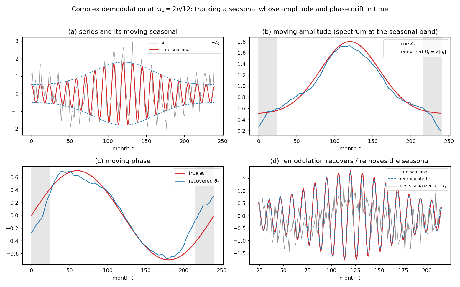
Fig. 25 Figure 1. Complex demodulation at \(\omega_0 = 2\pi/12\) of a synthetic monthly series
\(x_t = A_t\cos(\omega_0 t + \phi_t) + (\text{10-yr cycle}) + (\text{6-mo harmonic}) +
\text{noise}\). (a) the series with its moving seasonal and the envelope \(\pm A_t\);
(b) the recovered amplitude \(R_t = 2|d_t|\) tracks the true \(A_t\) — a moving spectrum at
the seasonal band (shaded ends are corrupted by the filter); (c) the recovered phase
\(\theta_t\) tracks the true \(\phi_t\); (d) the remodulated band \(r_t\) recovers the seasonal,
and \(x_t - r_t\) is the deseasonalized series. The low-pass filter is a length-\(25\) moving
average iterated twice (Bartlett window). Generated by
code/ch41_demod_seasonal.py.#
Locating a spectral peak#
The phase of a demodulate carries information about where the power actually sits, a fact Godfrey (1965, eqs. 2.9–2.12) exploited to locate peaks. Suppose the series contains a pure component at an unknown frequency \(\omega_1\), \(x_t = a\cos\omega_1 t\), and we demodulate at a trial frequency \(\omega_0\). Then \(x_t e^{-i\omega_0 t}\) has a slow part proportional to \(e^{i(\omega_1-\omega_0)t}\), so after low-pass filtering
The demodulate phase is linear in time, with slope equal to the offset between the trial frequency and the true peak. Demodulating just below the peak gives a phase that climbs at a constant rate; just above, it falls; exactly on the peak it is flat. This converts peak-finding into reading the slope of a straight line, and it warns that a demodulate centered slightly off a sharp spectral peak will appear to drift in phase even though the underlying process is perfectly stationary — a trap to keep in mind when interpreting moving phases. Figure 2 illustrates the three cases.
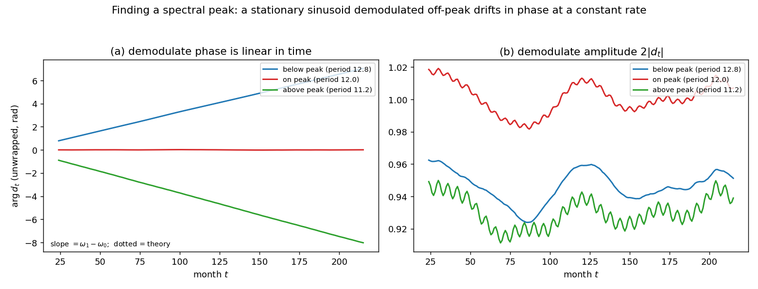
Fig. 26 Figure 2. A stationary sinusoid of period \(12\) demodulated at three trial frequencies.
(a) the unwrapped demodulate phase is linear in time with slope \(\omega_1-\omega_0\) (dotted
theory lines lie under the data): demodulating below the peak gives a rising line, above the
peak a falling line, on the peak a flat one. (b) the demodulate amplitude \(2|d_t|\) is largest
on the peak. Generated by
code/ch41_demod_peak.py.#
A moving cross spectrum#
Demodulation extends to two series, producing a cross spectrum that is local in time. Demodulate \(y_t\) and \(x_t\) at the same \(\omega_0\) to get \(d^y_t\) and \(d^x_t\), and form the local cross product, smoothed over a moving window \(\langle\cdot\rangle\) in time:
This is the time-varying analog of the cross spectrum \(g_{yx}(e^{-i\omega_0})\), and from it come the same three real summaries introduced in The Cross Spectrum — now functions of \(t\):
The phase converts to a lead of \(y\) over \(x\), measured in time units, by \(\tau_t = \theta^{yx}_t(\omega_0)/\omega_0\); at the twelve-month frequency this is a lead in months, the conversion Sargent reports in his Table 2. The extra time-smoothing \(\langle\cdot\rangle\) in (532) is essential: without it, the squared coherence of a single demodulate pair is identically \(1\), exactly as the raw squared coherence of one realization is (the same point made for the spectrum in The Spectrum). Smoothing over a window short enough to preserve genuine movement but long enough to average out noise is the cross-spectral counterpart of the bandwidth choice for \(W(L)\).
Figure 3 demodulates two seasonal series whose lead and whose strength of comovement both drift through time.
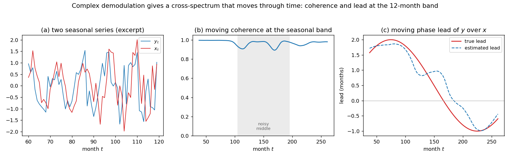
Fig. 27 Figure 3. A moving cross spectrum at the seasonal band. Two monthly series share a
twelve-month seasonal, but the lead of \(y\) over \(x\) drifts and their comovement is degraded
by incoherent seasonal noise that is strongest in the middle of the sample. (a) an excerpt of
the two series; (b) the moving coherence (533) dips where the comovement is noisiest;
(c) the moving phase lead \(\tau_t = \theta^{yx}_t/\omega_0\) in months tracks the true drifting
lead (and wobbles where coherence is low). Generated by
code/ch41_demod_cross.py.#
Application: the changing seasonal in interest rates, 1951–1960#
Sargent (1968) studied monthly rates on eleven money- and capital-market instruments — three-month Treasury bills, governments of one to twenty years’ maturity, commercial paper, and Moody’s Aaa and Baa corporates — over 1951–1960, working with first differences to remove the trend. The ordinary spectral and cross-spectral statistics (coherence, phase, gain of The Cross Spectrum) revealed strong seasonal peaks at twelve months and its harmonics, generally declining in amplitude as maturity lengthens, and a tendency for the longer rates to lead the bill rate, the lead increasing as maturity increases — a pattern reminiscent of Macaulay’s (1938) finding for 1890–1913.
The seasonal peaks raised a question that stationary cross-spectra could not settle: were the seasonal in the long–short rate spread and the seasonal in the average maturity of the publicly held debt moving together, as a segmented-markets or hedging theory of the term structure would predict? To answer it Sargent turned to complex demodulation, “the relatively new tool” of his title’s program. He demodulated the rate spread and the average maturity at the twelve-month cycle and its first three harmonics, using the iterated moving-average low-pass filter of (528) with \(m=18\), and then remodulated ((529)–(530)) to construct the estimated seasonal of each series as a function of calendar time. The resulting moving seasonals — his Figure 3 — show the seasonal pattern of the bill rate, of the ten-year-minus-bill spread, and of the average maturity evolving month by month from 1954 to 1963, with amplitudes that grow and shrink across the decade rather than repeating identically.
Reading the demodulates jointly delivered the economic conclusion. The seasonals in the rate spread and in the average maturity were close in phase over the first several years, consistent with the two being directly related at the seasonal frequencies; the moving cross spectrum ((532)–(533), his Table 2) showed high coherence at the seasonal and a small phase difference, with the rate spread leading the average maturity by one to five months at the lower frequencies. Sargent read this as the Treasury adjusting the maturity structure of the debt in response to the spread — lengthening maturity when long rates were low — while the tight seasonal comovement was at best transitory. None of this is visible in a single stationary spectrum; it requires the local-in-time amplitude and phase that demodulation provides.
A replication on FRED data#
We can re-run Sargent’s exercise on data anyone can download. The variables he used are
interest rates, which the St. Louis Fed publishes not seasonally adjusted — exactly
what a study of the seasonal requires. The closest monthly NSA series reaching back to the
1950s are the three-month Treasury bill rate (TB3MS, from 1934), the one-, five-, and
twenty-year Treasury constant-maturity rates (GS1, GS5, GS20, from April 1953), the
ten-year rate (GS10), and Moody’s Aaa and Baa corporate yields (AAA, BAA, from 1919).
Following Sargent we first-difference each rate to remove the trend, then demodulate at the
twelve-month frequency \(\omega_0 = 2\pi/12\) and its first three harmonics with the iterated
moving-average filter of (528) (\(m=18\), \(r=2\)).
Figure 4 reproduces his three seasonal findings. Panel (a) — a smoothed periodogram of the differenced bill rate over 1951–1972 — shows the sharp peaks at periods \(12,6,4,3\) months that establish the seasonal (his Figure 1a). Panel (b) is the moving seasonal component \(s_t\) of (530), the running analog of his Figure 3a. Panel (c) measures, for each maturity, the local seasonal share — the variance of the remodulated seasonal band as a fraction of the variance of the differenced rate — over 1957–1967, and finds it declining with maturity (bill \(0.27\), one-year \(0.19\), five-year \(0.16\), twenty-year \(0.16\)), Sargent’s finding (b). The volatility-normalized share is the honest way to compare across maturities and eras: the absolute seasonal swing in basis points is largest in the high-rate 1970s and early 1980s simply because every movement was larger then, but relative to total variation the bill-rate seasonal was strongest in the 1950s–60s and has largely faded from short rates since the mid-1980s.
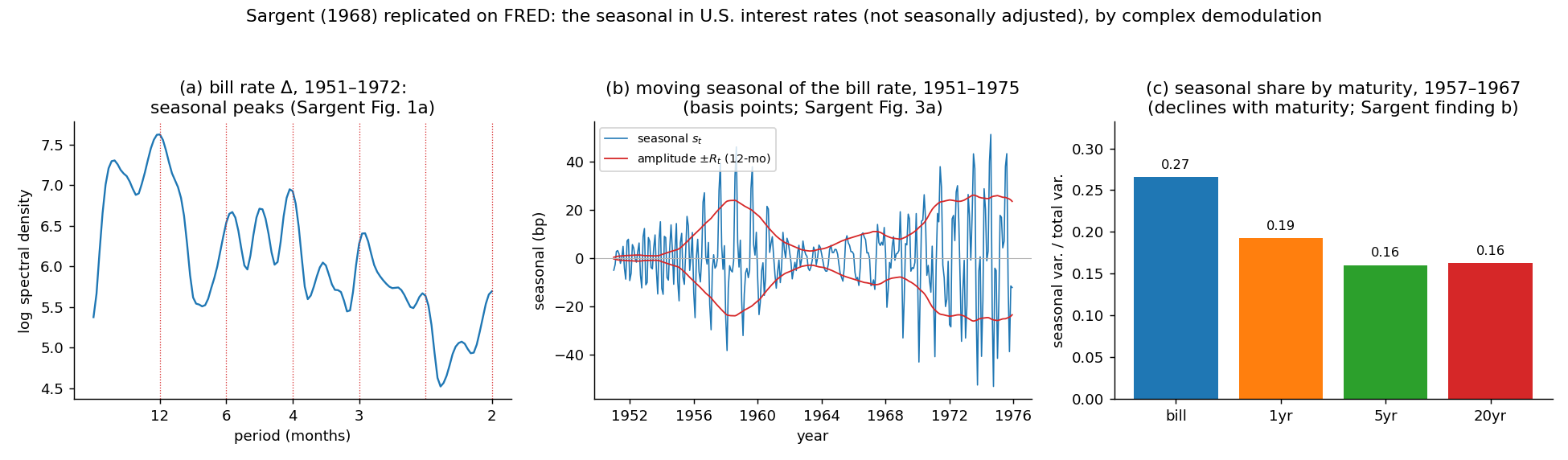
Fig. 28 Figure 4. Sargent (1968) replicated on FRED. (a) The spectral density of the
first-differenced three-month bill rate (TB3MS, NSA) over 1951–1972 has peaks at the
seasonal periods \(12,6,4,3,2\) months. (b) The moving seasonal \(s_t = \sum_{k=1}^{4}
r_t(k\omega_0)\) of the differenced bill rate, 1951–1975, with the moving amplitude \(\pm R_t\)
of the twelve-month fundamental (basis points; his Figure 3a). (c) The seasonal share by
maturity over 1957–1967 declines as maturity lengthens (his finding b). Generated by
code/ch41_fred_seasonal.py.#
The moving cross spectrum reproduces his cross-spectral results just as closely. Figure 5 demodulates the differenced bill and ten-year rates at the seasonal and forms (532)–(533) over 1953–1975. The coherence is very high throughout (median \(0.97\) — Sargent: “almost all very high”), and the phase lead of the bill over the ten-year is negative, hovering around \(-1.5\) months: the ten-year rate leads the bill rate at the seasonal by about a month and a half. Sargent’s Table 1 reports a phase of \(-0.7978\) radians for this pair at period 12, which is \(-0.7978 \times 12/(2\pi) = -1.52\) months; our demodulation gives a median of \(-1.49\). That the longer rate should lead the shorter at the seasonal is the pattern Sargent traced back to Macaulay (1938) and read as evidence that the seasonal was, to a degree, forecast and impounded in the longer rate.
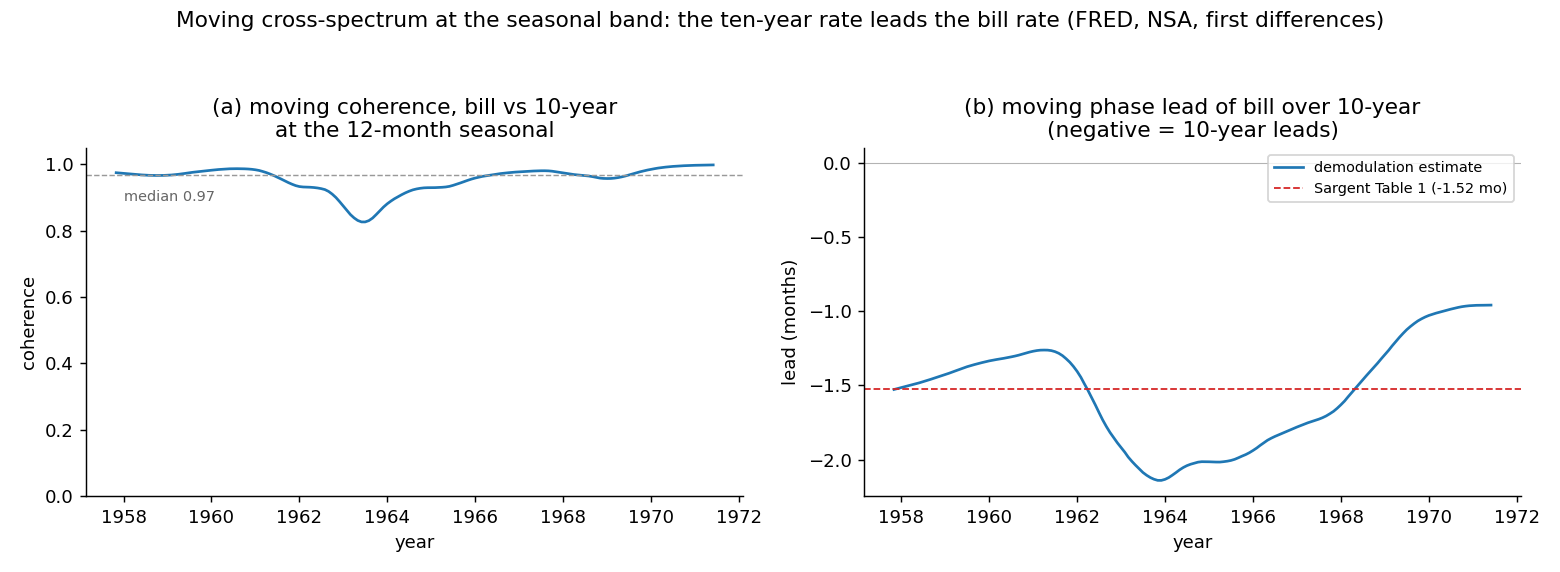
Fig. 29 Figure 5. Moving cross spectrum of the first-differenced bill (TB3MS) and ten-year
(GS10) rates at the twelve-month band, 1953–1975, both NSA. (a) the moving coherence
(533) stays near \(0.97\); (b) the moving phase lead \(\theta^{yx}_t/\omega_0\) of the bill
over the ten-year is about \(-1.5\) months — the ten-year leads — matching Sargent’s Table 1 value
of \(-1.52\) months (red dashed). Generated by
code/ch41_fred_cross.py.#
The one piece of Sargent’s study we cannot reproduce from FRED is the average maturity of the publicly held debt, which is not available as a monthly series back to the 1950s; the bill-versus-long comparison above stands in for the cross-spectral half of his analysis.
Exercise#
Exercise 58 (Detecting a seasonal break)
Many seasonal patterns shift abruptly when an institution changes — a payment rule, a market convention, a policy regime. Complex demodulation should reveal such a break as a jump in the demodulate amplitude or a kink in its phase.
Simulate a monthly series with a twelve-month seasonal that breaks at \(t^\star\): let the amplitude jump (say from \(A=1\) to \(A=2\)) and the phase shift (say by \(\phi=\pi/2\)) at \(t=t^\star\), and add a low-frequency cycle and white noise so the seasonal is not obvious in the raw plot:
\[x_t = A(t)\cos\!\big(\tfrac{\pi}{6}t + \phi(t)\big) + 0.5\cos\!\big(\tfrac{2\pi}{120}t\big) + \varepsilon_t .\]Demodulate at \(\omega_0=\pi/6\) with the iterated moving-average filter (528) (\(r=2\); try \(m=6\) and \(m=18\)). Plot \(R_t = 2|d_t|\) and \(\theta_t = \arg d_t\) and locate the break. How does the apparent sharpness of the break in \(R_t\) depend on \(m\)? Relate your answer to the time–frequency trade-off and to the \(\sim rm\) observations lost at each end.
Remodulate ((529)) to extract the seasonal component on each side of the break and confirm that \(x_t - r_t\) is free of the twelve-month oscillation.
Harder. Add a second series \(z_t\) that shares the seasonal but whose break is lagged by three months, and use the moving cross spectrum (532)–(533) to estimate the coherence and the phase lead of \(x\) over \(z\) before and after \(t^\star\). Verify that the estimated lead \(\theta^{xz}_t/\omega_0\) recovers the three-month lag, and watch the coherence fall transiently around the break where the two seasonals are momentarily out of step.
The scripts behind Figure 1 and Figure 3 provide a lowpass,
demodulate, and cross-spectral template you can adapt.
References#
R. B. Blackman and John W. Tukey. The Measurement of Power Spectra. Dover, New York, 1959.
M. D. Godfrey. An exploratory study of the bi-spectrum of economic time series. Journal of the Royal Statistical Society, Series C (Applied Statistics), 14(1):48–69, 1965.
Frederick R. Macaulay. The Movements of Interest Rates, Bond Yields and Stock Prices in the United States Since 1856. National Bureau of Economic Research, New York, 1938.