Seasonal Adjustment and Forecasting Geometric Distributed Leads

A stochastic process \(x_t\) is said to have an important seasonal component if its spectral density has peaks in the vicinity of the seasonal frequencies, meaning that the process has a substantial portion of its variance occurring over the seasonal frequencies. It is a common practice to “seasonally adjust” the series in order to remove the seasonal components. Unless the seasonal components are thought mainly to reflect measurement errors that are unrelated to economic activity, seasonal adjustment is typically misleading. We briefly indicate how using seasonally adjusted data can distort analysis. We have often encountered, and shall encounter even more often later, models in which economic agents decide to make an endogenous variable \(y_t\) a geometric sum of expected future values of a variable \(x_t\):

(364)\[y_t=P_t\sum_{j=0}^\infty \lambda^j x_{t+j},\]

where \(P_t\) is the linear least squares projection operator conditioned on \([x_t,x_{t-1},\ldots]\). Now let \(x_t\) be a covariance stationary stochastic process with Wold representation

(365)\[x_t=c(L)\epsilon_t,\]

Let \(x_t\) have a substantial seasonal component, say reflecting weather or seasonal movements in tastes (Christmas and Easter). These seasonal movements are assumed not to be due to measurement error, but are truly occurring in the process that \(x_t\) is measuring. We have seen above that (364) and (365) imply that \(y_t\) will obey

(366)\[y_t=\left[\frac{c(L)-\lambda c(\lambda)L^{-1}}{1-\lambda L^{-1}}\right]\epsilon_t,\]

or

(367)\[y_t=\left[\frac{1-\lambda c(\lambda)c(L)^{-1}L^{-1}}{1-\lambda L^{-1}}\right]x_t,\]

Now suppose that an analyst has seasonally adjusted \(x_t\) to obtain a process \(x_t^a\). Typically this is accomplished by taking

(368)\[x_t^a=h(L)x_t\]

where \(h(L)\) is a long two-sided filter that attenuates (but does not completely eradicate) power at the seasonal frequencies. We indicated how to construct such a filter in Section 6 above. Typically, these seasonal adjustment filters are symmetric with \(h_j=h_{-j}\). (See Exercise 34 and Section 6.)

If the economic agent is choosing \(y_t\) to obey (367), then \(y_t\) is related to the seasonally adjusted series \(x_t^a\) by

\[ h(L)y_t=\left[\frac{1-\lambda c(\lambda)c(L)^{-1}L^{-1}}{1-\lambda L^{-1}}\right]h(L)x_t, \]

or

(369)\[h(L)y_t=\left[\frac{1-\lambda c(\lambda)c(L)^{-1}L^{-1}}{1-\lambda L^{-1}}\right]x_t^a.\]

Suppose that seasonally adjusted data on \(y_t\) denoted \(y_t^a\) are created via the same filter \(h(L)\) used to create \(x_t^a\) so that

(370)\[y_t^a=h(L)y_t.\]

In view of (370), (369) becomes

(371)\[y_t^a=\left[\frac{1-\lambda c(\lambda)c(L)^{-1}L^{-1}}{1-\lambda L^{-1}}\right]x_t^a.\]

where \(c(L)\) is the Wold representation for the seasonally unadjusted series \(x_t\), given in (365). (In Sims (1974) and Exercise 42, the effects are studied of adjusting \(y_t\) and \(x_t\) by using different seasonal filters.)

If agents are behaving according to (367) or (371), the restrictions across the \(y_t^a\) and \(x_t^a\) processes cannot be computed from knowledge of the autoregression for \(x_t^a\) alone, without knowledge of the seasonal adjustment filter \(h(L)\). If one routinely applies the Hansen-Sargent formula (282) based on using the moving average or autoregressive representation for the seasonally adjusted series, an error is committed, whose nature we now briefly explore. We continue to suppose that economic agents are actually choosing \(y_t\) to satisfy (364) and therefore (367). Suppose that the economist mistakenly uses the seasonally adjusted data to create the model

(372)\[y_t=P_t \sum_{j=0}^\infty \lambda^j x^a_{t+j}\]

where now \(P_t\) denotes the least squares projection on the space \([x_t^a, x^a_{t-1},\ldots]\). To deduce the implications of model (372), we need the Wold representation of \(x_t^a\),

(373)\[x_t^a=d(L)a_t,\quad d(L)=\sum_{j=0}^\infty d_jL^j\]

\[ a_t = x^a_t - P[x_t^a| x^a_{t-1},x^a_{t-2},\ldots] \]

Now \(d(L)\) of (373) is related to \(c(L)\) of (365) by the spectral factorization equation

(374)\[\sigma^2_ad(L)d(L^{-1}) =\sigma_\epsilon^2h(L)h(L^{-1})c(L)c(L^{-1})\]

where \(\sigma^2_a=Ea_t^2\), \(\sigma_\epsilon^2=E\epsilon_t^2\), and \(d(L)\) has all of its zeros outside the unit circle. Note that in general \(h(L)\) is two-sided in powers of \(L\), and that \(d(L) \neq h(L)c(L)\). Equations (372) and (373) imply that

(375)\[y_t=\left[\frac{1-\lambda d(\lambda)d(L)^{-1}L^{-1}}{1-\lambda L^{-1}}\right]x_t^a.\]

Using \(x_t^a=h(L)x_t\), we have that

(376)\[y_t=\left[\frac{1-\lambda d(\lambda)d(L)^{-1}L^{-1}}{1-\lambda L^{-1}}\right]h(L)x_t.\]

A comparison of equations (367), (374), and (376) shows how (376) misspecifies the relationship between \(y_t\) and \(\{x_t\}\) if agents are responding to forecasts of the seasonally unadjusted series while the economist attributes to agents their responding to forecasts of the seasonally adjusted series. Alternatively, a comparison of (369) with (375) shows how deducing the cross-equation restrictions on the basis of the seasonally adjusted data misspecifies the relationship between \(y_t^a\) and \(x_t^a\). Continuing to suppose that \(y_t^a=h(L)y_t\), applying \(h(L)\) to both sides of (375) implies that

(377)\[y_t^a=h(L)\left[\frac{1-\lambda d(\lambda)d(L)^{-1}L^{-1}}{1-\lambda L^{-1}}\right]x_t^a.\]

whereas the actual value of \(y_t^a\) is determined by the right side of (369).

We illustrate these calculations as follows. For monthly U.S. money supply (M2) for the period 1959 to the present (Sargent’s original used 1959:1–1986:2) we constructed an 18th order autoregression for both seasonally adjusted and seasonally unadjusted M2. The spectral densities of seasonally adjusted and unadjusted M2 are reported in Figure 8. Notice the dips in the spectral density of the adjusted series at the seasonal frequencies (see Exercise 34). The autoregressive coefficients are plotted for seasonally adjusted and unadjusted series in Figure 9. In Figure 10, we report the values of the two filters in \(x\) associated with (371) and (375); namely,

\[ b^{nsa}(L)=\frac{1-\lambda c(\lambda)c(L)^{-1}L^{-1}}{1-\lambda L^{-1}}, \qquad b^{sa}(L)=\frac{1-\lambda d(\lambda)d(L)^{-1}L^{-1}}{1-\lambda L^{-1}} \]

where we set \(\lambda=0.9\) and where we have used the estimated autoregressive representations reported in Figure 9 for \(c(L)\) and \(d(L)\). Note the difference in \(b^{nsa}(L)\) and \(b^{sa}(L)\) in the vicinity of 12 lags. Figures 11 and 12 summarize the magnitude and phase of the transfer function from innovations in M2 to “\(y_t\)” that are associated with \(b^{sa}(L)\). That is, let the filters associated with the autoregressive representations be denoted as \(a^{sa}(L)\) and \(a^{nsa}(L)\), respectively. Then Figures 11–12 report the magnitude and phase of the transfer function

\[ k(e^{-i\omega}) \]

where \(k(L)\) is given by \(b^{nsa}(L)/a^{nsa}(L)\) or \(b^{sa}(L)/a^{sa}(L)\), respectively. (We write \(k\) rather than \(h\) here to avoid collision with the seasonal adjustment filter \(h(L)\) of (368).) Note the substantially different responses revealed in these figures.

Some of these ideas are explored further in Exercise 54 and Exercise 55.

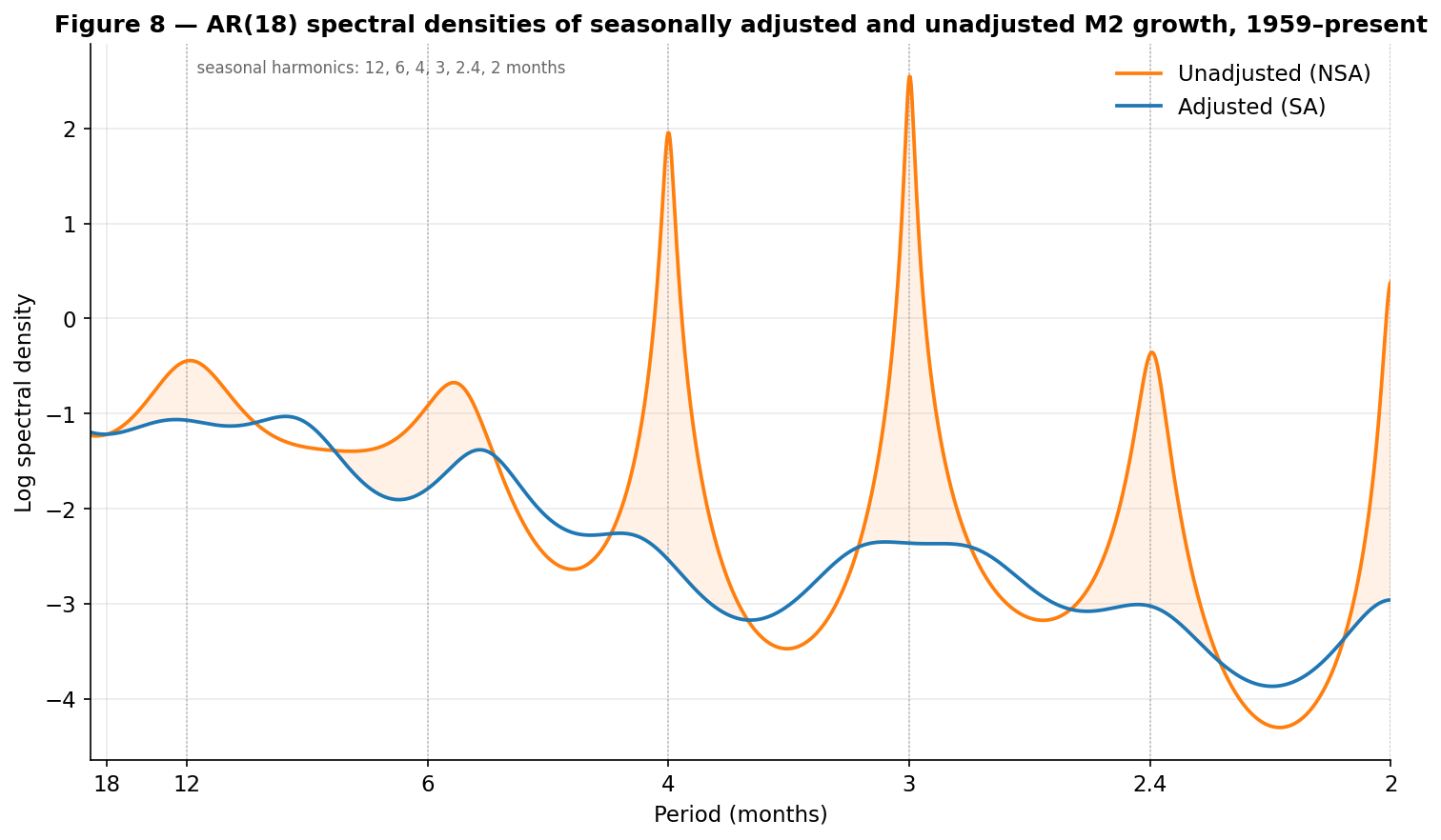
Fig. 17 Figure 8. AR(18) spectral densities of seasonally adjusted (M2SL) and unadjusted (M2NS) monthly M2 growth (\(\Delta\log M2\)), 1959–present (Sargent’s original used 1959:1–1986:2). An 18th-order autoregression is fit by OLS to each growth series; the curves are \(\log g(\omega) = \log\!\big(\sigma^2/|A(e^{-i\omega})|^2\big)\). (We fit the AR to the growth rate rather than the log level because log M2 is so close to a random walk — the level AR has \(\sum_k a_k \approx 0.9998\) — that the resulting near-unit-root pole at \(\omega=0\) would otherwise swamp the seasonal structure that is the point of these figures, especially in the transfer functions of Figures 11–12.) The unadjusted series shows sharp peaks at the seasonal periods (12, 6, 4, 3, 2.4, 2 months); seasonal adjustment carves matching dips there — the shaded gap is exactly the seasonal power removed. (Sargent’s caption reads “M1”; the text describes the construction with M2, which we follow.) Generated by code/fig8_m2_spectra.py.

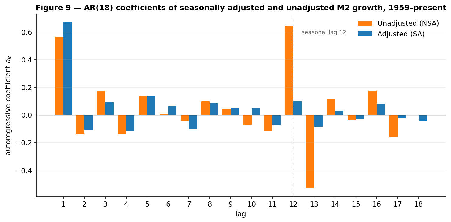
Fig. 18 Figure 9. OLS AR(18) coefficients \(a_1,\dots,a_{18}\) for unadjusted (M2NS) and adjusted (M2SL) monthly M2 growth, 1959–present. The unadjusted series carries pronounced seasonal coefficients at lags 12–14 that the adjusted series lacks (e.g. \(a_{12}\approx 0.64\) unadjusted versus \(0.10\) adjusted). Generated by code/fig9_m2_ar_coeffs.py.

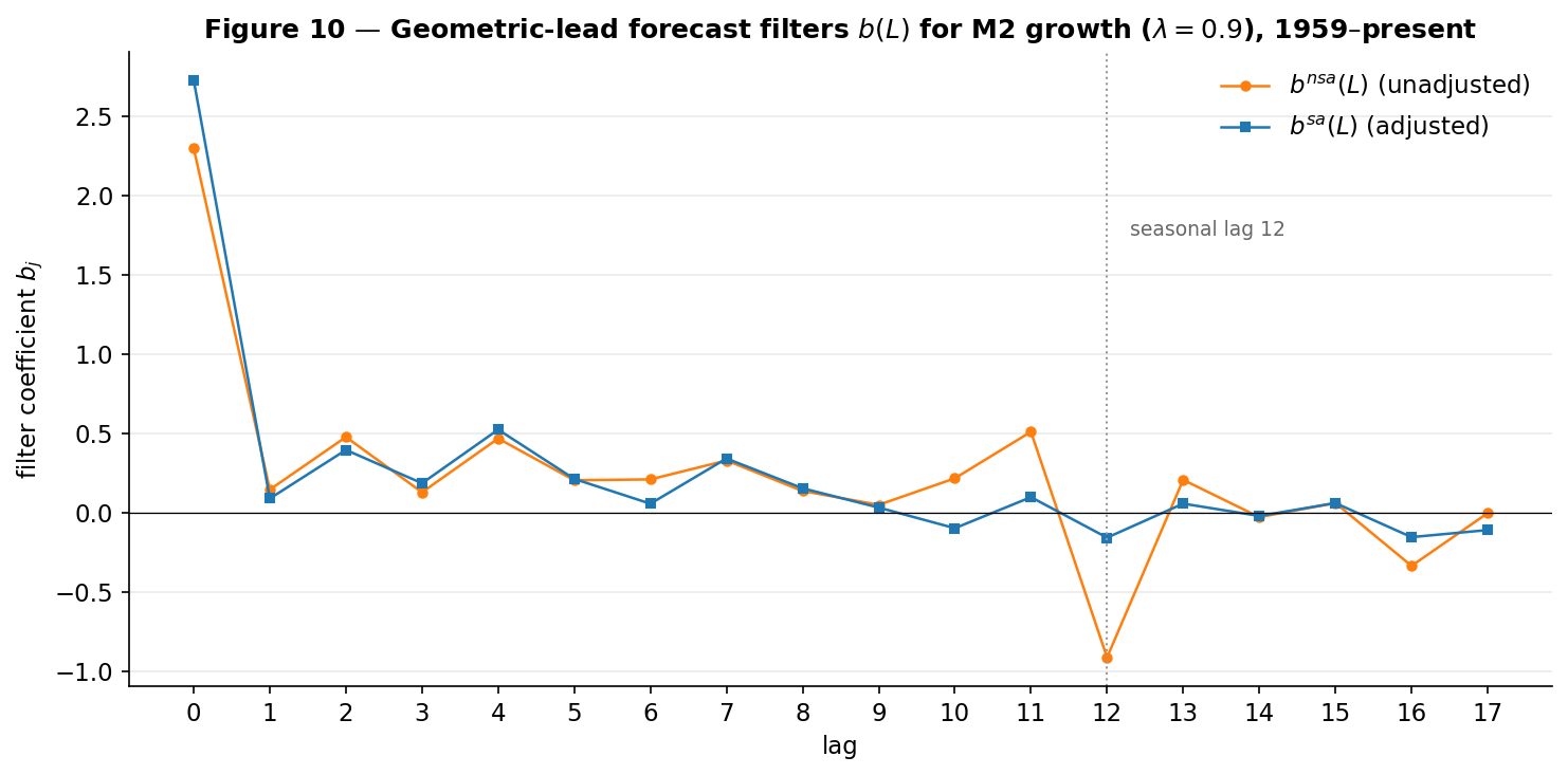
Fig. 19 Figure 10. Geometric-lead forecast filters \(b^{nsa}(L)\) and \(b^{sa}(L)\) (Hansen–Sargent formula, \(\lambda = 0.9\)) implied by the two AR(18) representations, for the projection \(y_t = P_t\sum_j \lambda^j x_{t+j}\). The filters agree at short lags but diverge sharply near lag 12: forecasting future unadjusted money inherits the seasonal autoregressive structure (the large spike at lags 12–13), which seasonal adjustment removes. Generated by code/fig10_m2_lead_filter.py.

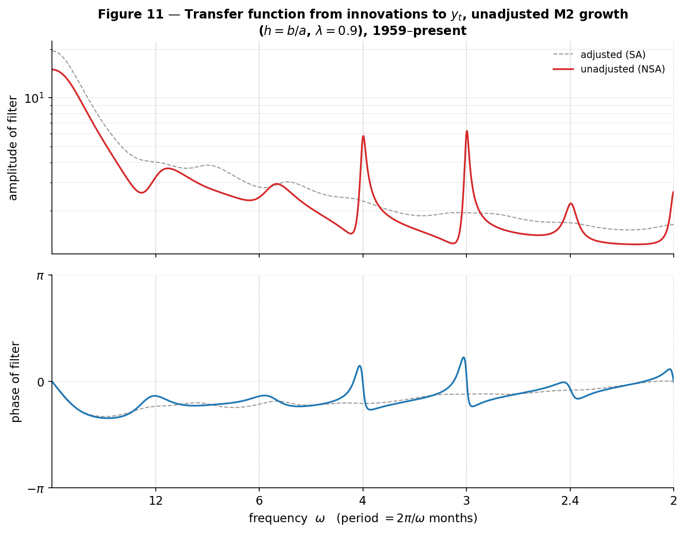
Fig. 20 Figure 11. Amplitude (log scale) and phase of the transfer function \(h(e^{-i\omega}) = b^{nsa}(e^{-i\omega})/a^{nsa}(e^{-i\omega})\) — from a money-growth innovation to the geometric-lead forecast \(y_t\) — for the unadjusted series (the adjusted case is overlaid faintly for comparison). The unadjusted response shows sharp resonance peaks at the seasonal frequencies (periods 12, 6, 4, 3, 2.4, 2 months), with matching jumps in the phase; the adjusted response is smooth there. Generated by code/fig11_12_m2_transfer.py.

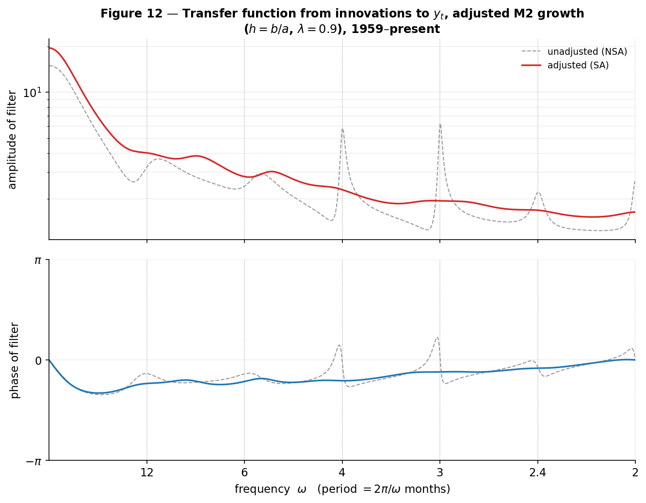
Fig. 21 Figure 12. The same transfer function for the adjusted series, \(h(e^{-i\omega}) = b^{sa}(e^{-i\omega})/a^{sa}(e^{-i\omega})\) (the unadjusted case overlaid faintly). Comparing Figures 11 and 12 reveals the “substantially different responses” Sargent emphasizes: away from the seasonal frequencies the two transfer functions nearly coincide, but at the seasonal frequencies the unadjusted filter has sharp resonances (and phase jumps) that seasonal adjustment removes. Generated by code/fig11_12_m2_transfer.py.