Analysis of Some Filters: The Slutsky Effect and Kuznets’s Transformations

Relation (200) can be used to show the famous “Slutsky effect” (1937). Slutsky considered the effects of starting with a white noise \(\epsilon_t\), taking a two period moving sum \(n\) times, and then taking first differences \(m\) times. That is, Slutsky considered the series

\[ Z_t = (1+L)(1+L)\cdots(1+L)\epsilon_t = (1+L)^n\epsilon_t \]

and

(233)\[y_t = (1-L)(1-L)\cdots(1-L)Z_t = (1-L)^m Z_t = (1+L)^n(1-L)^m\epsilon_t.\]

Applying (200) to (233), we have

(234)\[\begin{split}g_y(e^{-i\omega}) = (1+e^{i\omega})^n(1+e^{-i\omega})^n(1-e^{i\omega})^m(1-e^{-i\omega})^m\,\sigma_\epsilon^2 \\ = [(1+e^{i\omega})(1+e^{-i\omega})]^n\,[(1-e^{i\omega})(1-e^{-i\omega})]^m\,\sigma_\epsilon^2 \\ = [2+(e^{i\omega}+e^{-i\omega})]^n\,[2-(e^{i\omega}+e^{-i\omega})]^m\,\sigma_\epsilon^2 \\ = \sigma_\epsilon^2\, 2^n[1+\cos\omega]^n\, 2^m[1-\cos\omega]^m.\end{split}\]

Consider first the special case where \(m = n\). Then (234) becomes

(235)\[g_y(e^{-i\omega}) = \sigma_\epsilon^2\, 4^n[1 - \cos^2\omega]^n = \sigma_\epsilon^2\, 4^n[\sin^2\omega]^n.\]

On \((0, \pi)\), the spectrum of \(y\) has a peak at \(\omega = \pi/2\) since there \(\sin\omega = 1\). Notice that since \(\sin\omega \leq 1\), (235) implies that as \(n\) becomes large, the peak in the spectrum of \(y\) at \(\pi/2\) becomes sharp. In the limit, as \(n \to \infty\), the spectrum of \(y\) becomes a “spike” at \(\pi/2\), which means that \(y\) behaves like a cosine of angular frequency \(\pi/2\).

Similar behavior results for a fixed \(m/n\) as \(n\) becomes large where \(m \neq n\). Consider (234) and set \(dg_y(e^{-i\omega})/d\omega\) equal to zero in order to locate the peak in the spectrum:

\[\begin{split} dg_y/d\omega = \sigma_\epsilon^2\, 2^{m+n}\{n[1-\cos\omega]^m[1+\cos\omega]^{n-1}(-\sin\omega) \\ + m(1-\cos\omega)^{m-1}(\sin\omega)[1+\cos\omega]^n\} \\ = \sigma_\epsilon^2\, 2^{m+n}\sin\omega\{(1-\cos\omega)^{m-1}(1+\cos\omega)^{n-1} \\ [m(1+\cos\omega) - n(1-\cos\omega)]\}. \end{split}\]

This expression can equal zero on \((0, \pi)\) only if the expression in brackets equals zero:

\[ m(1+\cos\omega) - n(1-\cos\omega) = 0. \]

which implies

\[ \cos\omega = \frac{1-(m/n)}{1+(m/n)} \qquad \text{or} \qquad \omega = \cos^{-1}\!\left(\frac{1-(m/n)}{1+(m/n)}\right) \]

which tells us the frequency at which the spectrum of \(y\) attains a peak. For fixed \(m/n\), the spectrum of \(y\) approaches a spike as \(n \to \infty\). This means that as \(n \to \infty\), \(y\) tends to behave more and more like a cosine of angular frequency \(\cos^{-1}\!\left(\frac{1-(m/n)}{1+(m/n)}\right)\).

What Slutsky showed, then, is that by successively summing and then successively differencing a serially uncorrelated or “white-noise” process \(\epsilon_t\), a series with “cycles” is obtained.

Another use of (200) is in the analysis of transformations that have been applied to data. An example is Howrey’s (1968) analysis of the transformations used by Kuznets. Data constructed by Kuznets have been inspected to verify the existence of “long swings,” long cycles in economic activity of around twenty years. Before analysis, however, Kuznets subjected the data to two transformations. First, he took a five-year moving average:

\[ Z_t = \frac{1}{5}[L^{-2} + L^{-1} + 1 + L + L^2]\, X_t \equiv A(L)\, X_t. \]

Then he took the centered first difference of the (nonoverlapping) five-year moving average:

\[ y_t = Z_{t+5} - Z_{t-5} = [L^{-5} - L^5]\, Z_t = B(L)\, Z_t. \]

So we have that the \(y\)’s are related to the \(X\)’s by

\[ y_t = \frac{1}{5}[L^{-5} - L^5][L^{-2} + L^{-1} + 1 + L + L^2]\, X_t = A(L)B(L)\, X_t. \]

The spectrum of \(y\) is related to the spectrum of \(X\) by

\[ g_y(e^{-i\omega}) = A(e^{-i\omega})A(e^{i\omega})\, B(e^{-i\omega})B(e^{i\omega})\, g_x(e^{-i\omega}) \]

We have

\[ A(e^{-i\omega}) = \frac{1}{5}\sum_{j=-2}^{2} e^{-i\omega j} = \frac{1}{5}\frac{e^{i\omega 2} - e^{-i\omega 3}}{1 - e^{-i\omega}} \]

Thus,

\[\begin{split} A(e^{-i\omega})A(e^{i\omega}) = \frac{\left(\frac{1}{5}\right)^2(e^{i\omega 2}-e^{-i\omega 3})(e^{-i\omega 2}-e^{i\omega 3})} {(1-e^{-i\omega})(1-e^{i\omega})} \\ = \frac{\left(\frac{1}{5}\right)^2(2-(e^{i\omega 5}+e^{-i\omega 5}))} {2-(e^{i\omega}+e^{-i\omega})} \\ = \frac{\left(\frac{1}{5}\right)^2 2(1-\cos 5\omega)}{2(1-\cos\omega)} = \frac{\left(\frac{1}{5}\right)^2(1-\cos 5\omega)}{1-\cos\omega}. \end{split}\]

Next, we have \(B(e^{-i\omega}) = (e^{+i\omega 5} - e^{-i\omega 5})\), so that

\[\begin{split} B(e^{i\omega})B(e^{-i\omega}) = (e^{i\omega 5} - e^{-i\omega 5})(e^{-i\omega 5} - e^{i\omega 5}) \\ = (2-(e^{i\omega 10}+e^{-i\omega 10})) = 2(1-\cos 10\omega). \end{split}\]

So it follows from (200) that

\[ g_y(e^{-i\omega}) = \frac{\left(\frac{1}{5}\right)^2(1-\cos 5\omega)\cdot 2}{(1-\cos\omega)}(1-\cos 10\omega)\, g_x(e^{-i\omega}) = G(\omega)\, g_x(e^{-i\omega}), \]

where \(G(\omega) = 2\left[\left(\frac{1}{5}\right)^2(1-\cos 5\omega)(1-\cos 10\omega)/(1-\cos\omega)\right]\). The term \(G(\omega)\) is graphed in Figure 3. It has zeros at values where \(\cos 5\omega = 1\) and where \(\cos 10\omega = 1\). The first condition occurs on \([0, \pi]\) where

\[ 5\omega = 0,\, 2\pi,\, 4\pi, \qquad \omega = 0,\, \tfrac{2}{5}\pi,\, \tfrac{4}{5}\pi. \]

The condition \(\cos 10\omega = 1\) occurs on \([0, \pi]\) where

\[ 10\omega = 0,\, 2\pi,\, 4\pi,\, 6\pi,\, 8\pi,\, 10\pi \qquad \text{or} \qquad \omega = 0,\, \tfrac{1}{5}\pi,\, \tfrac{2}{5}\pi,\, \tfrac{3}{5}\pi,\, \tfrac{4}{5}\pi,\, \pi. \]

So \(G(\omega)\) has zeros at \(\omega = 0,\, \frac{1}{5}\pi,\, \frac{2}{5}\pi,\, \frac{3}{5}\pi,\, \frac{4}{5}\pi,\, \pi\).

From the graph of \(G(\omega)\), it follows that even if \(X_t\) is a white noise, a \(y\) series generated by applying Kuznets’s transformations will have a large peak at a low frequency, and hence will seem to be characterized by “long swings.” These long swings are clearly a statistical artifact; i.e., they are something induced in the data by the transformation applied and not really a characteristic of the economic system. With annual data, the biggest peak in Figure 3 corresponds to a cycle of about \(20\frac{1}{4}\) years which is close to the \(20\) year cycle found by Kuznets. Howrey’s observations naturally raise questions about the authenticity of the long swings identified by studying the data used by Kuznets.

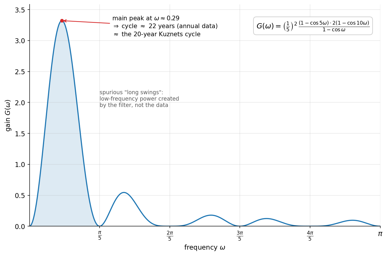
Fig. 9 Figure 3. The squared gain \(G(\omega)\) of Kuznets’s two-step transformation (a five-year moving average followed by a centered five-year difference), with zeros at \(\omega = 0, \tfrac{\pi}{5}, \tfrac{2\pi}{5}, \tfrac{3\pi}{5}, \tfrac{4\pi}{5}, \pi\). Even when the input \(X_t\) is white noise (a flat spectrum), the filter creates a large peak at a low frequency, so the output appears to contain “long swings.” The main lobe peaks at \(\omega \approx 0.29\), i.e. a cycle of roughly 22 years — close to the \(\approx 20\)-year cycle Kuznets reported. (Sargent’s original, reading the peak off the hand-drawn figure, gives \(\approx 20\tfrac{1}{4}\) years.) Generated by code/fig3_kuznets_gain.py.