A Small Kit of \(h(e^{-i\omega})\)’s

In order to provide some feel for the effects of the various commonly used filters, Figure 4 reports the amplitude and phase of \(h(e^{-i\omega})\) for various \(h(L)\) lag distributions.

We have already calculated that for \(h(L)=1-L\),

\[ h(e^{-i \omega})=2e^{i(\pi /2-\omega /2)}\sin(\omega /2), \]

as the graphs confirm.

For \(h(L)=1+L\), it is straightforward to calculate

\[ h(e^{-i\omega})=1+e^{-i\omega}=e^{-i\omega/2}(e^{+i\omega/2}+e^{-i\omega/2})=2e^{-i\omega/2}\cos (\omega/2), \]

which again agrees with our graphs.

Notice that for \(h(L)=(1-t_1 L - t_2 L^2)^{-1}\), we have chosen \((t_1,t_2)\) in the regions of peaked spectra of our Figure 2. Notice that as required, \(h(e^{-i\omega})\) is characterized by peaks. (See Figure 2.)

Figure 4 collects the amplitude \(|h(e^{-i\omega})|\) and phase \(\arg h(e^{-i\omega})\) of a kit of commonly used filters, grouped by family. All are generated by code/fig4_filter_kit.py, which evaluates \(h(e^{-i\omega}) = \mathrm{num}(e^{-i\omega})/\mathrm{den}(e^{-i\omega})\) for \(\omega \in [0, \pi]\).

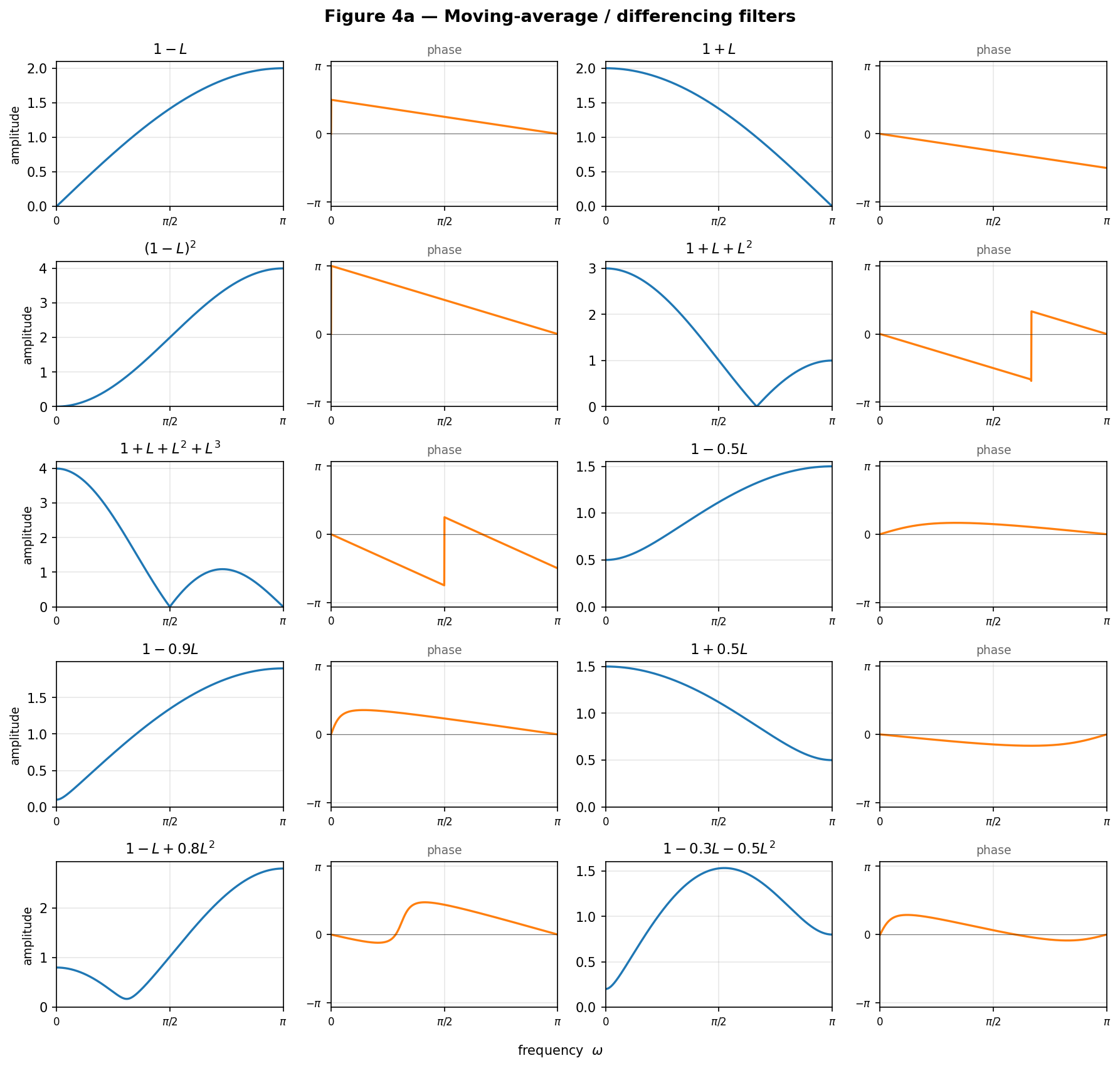
Fig. 10 Figure 4a. Moving-average / differencing filters. Note that \(1 - L\) (a first difference) suppresses low frequencies and amplifies high ones, while \(1 + L\) does the reverse; raising a filter to a power sharpens its effect.

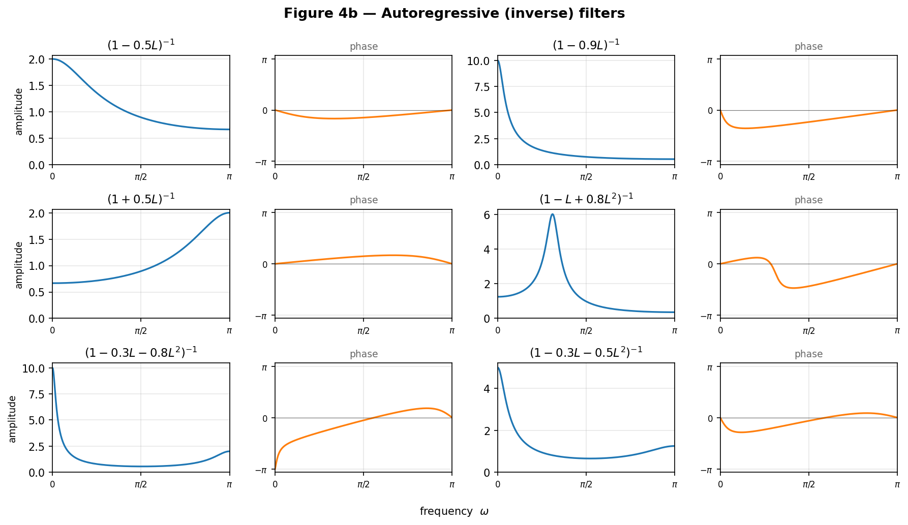
Fig. 11 Figure 4b. Autoregressive (inverse) filters. The filters \((1 - t_1 L - t_2 L^2)^{-1}\) use \((t_1, t_2)\) from the peaked-spectrum region of Figure 2; as required, \(h(e^{-i\omega})\) then displays a peak — e.g. \((1 - L + 0.8L^2)^{-1}\) shows a sharp resonance at an interior frequency.

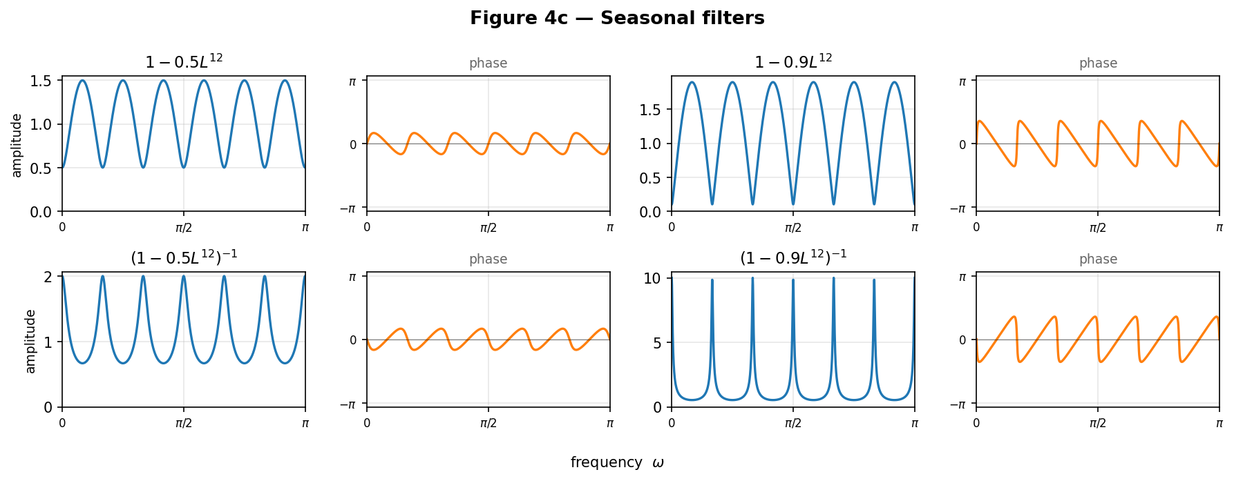
Fig. 12 Figure 4c. Seasonal filters in \(L^{12}\). Over \([0, \pi]\) the amplitude shows six ripples (the seasonal harmonics); \((1 - 0.9L^{12})^{-1}\) produces sharp peaks at the seasonal frequencies, the comb-like response characteristic of seasonal autoregressions.