Representation Theory

So far we have generally started with a white noise \(\epsilon_t\), as a building block and considered constructing a stochastic process \(x_t\), via a transformation

\[ x_t = B(L)\epsilon_t \]

In this section we reverse this procedure and start by assuming that we have a covariance stationary process \(x_t\), with covariogram \(c(\tau)\). We then show that associated with every such process \(\{x_t\}\) is a white-noise process \(\{\epsilon_t\}\) that is its fundamental building block. One purpose of this construction is to convey the sense in which the models we have been studying are quite general ones for covariance stationary processes.

Suppose that we have a covariance stationary stochastic process \(x_t\), with covariogram \(c(\tau)\) and mean zero. We think of forming a sequence of linear least squares projections (the regressions of Chapter X) of \(x_t\), against a sequence of expanding sets of past \(x\)’s, \(\{x_{t-1}, x_{t-2}, \ldots, x_{t-n}\}\):

\[ \hat{x}^n_t = \sum_{i=1}^n a_i^n x_{t-i} = P[x_t | x_{t-1}, \ldots , x_{t-n}] \qquad \text{or} \qquad x_t = \hat{x}_t^n + \epsilon_t^n \]

where \(E \epsilon_t^n x_{t-i} = 0 \, \text{for}\, i = 1, \ldots, n\) by the orthogonality principle. These orthogonality conditions uniquely determine the projection \(\hat{x}^n_t = \sum_{i=1}^n a_i^n x_{t-i}\). The population covariogram \(c(\tau)\) contains all of the information necessary to calculate the \(a_i^n\) from the least squares normal equations.[1]

As \(n\) is increased toward infinity, it is possible to show that the sequence of projections \(\{ \hat{x}^n_t\}\) converges to a random variable \(\hat{x}_t\) in the “mean square” sense that[2]

\[ \lim_{n \to \infty} E(\hat{x}_t - \hat{x}_t^n)^2 = 0 \]

This means that for any \(\delta > 0\), we can find an \(N(\delta)\) such that

\[ E(\hat{x}_t - \hat{x}_t^m)^2 < \delta \]

for all \(m > N(\delta)\), so that in the mean square sense, we can approximate arbitrarily well the projection on the space spanned by the infinite set of lagged \(x\)’s with the projection of \(x_t\), on a suitable finite set of lagged \(x\)’s.[3] We write the projection of \(x_t\) on the space spanned by the infinite set \((x_{t-1}, x_{t-2},\ldots)\) as

\[ \hat{x}_t = P[x_t | x_{t-1}, x_{t-2}, \ldots] \]

and have the decomposition of \(x_t\) as

(239)\[x_t = P[x_t | x_{t-1}, x_{t-2}, \ldots] + \epsilon_t\]

where \(\epsilon_t\) is a least squares residual that obeys the orthogonality condition \(E\epsilon_t x_{t-i} = 0\) for all \(i \geq 1\). In mean square \(\epsilon_t\) is the limit as \(n \to \infty\) of \(\epsilon_t^n\), i.e., \(\lim_{n \to \infty} E(\epsilon_t - \epsilon_t^n)^2 = 0\).

We can now state an important decomposition theorem due to Wold.[4]

Theorem 2 (Wold’s decomposition)

Let \(\{ x_t \}\) be any covariance stationary stochastic process with \(E x_t = 0\). Then it can be written as

\[ x_t = \sum_{j=0}^{\infty} d_j \epsilon_{t-j} + \eta_t \]

where \(d_0\) = 1 and where \(\sum_{j=0}^{\infty} d_j^2 < \infty\), \(E\epsilon_t^2 = \sigma^2 \geq 0\), \(E\epsilon_t \epsilon_s = 0\) for \(t \neq s\) (so that \(\{ \epsilon \}\) and \(\{ \eta_t \}\) are processes that are orthogonal at all lags); and \(\{\eta_t\}\) is a process that can be predicted arbitrarily well by a linear function of only past values of \(x_t\), i.e., \(\eta_t\) is linearly deterministic. Furthermore, \(\epsilon_t = x_t - P[x_t | x_{t-1}, x_{t-2}, \ldots].\)

Proof. We let \(\epsilon_t\) be the same \(\epsilon_t\) as appears in (239), so that

\[ \epsilon_t = x_t - P[x_t | x_{t-1}, x_{t-2}, \ldots]. \]

So \(\epsilon_t\), is the error or “innovation” in predicting \(x_t\), from its own past. Now \(\epsilon_t\) is orthogonal to \(\{x_{t-1}, x_{t-2}, \ldots \}\), by the orthogonality principle. But \(\epsilon_{t-s}\) is a linear combination of past \(x\)’s:

\[ \epsilon_{t-s} = x_{t-s} - P[x_{t-s} | x_{t-s-1}, \ldots] \]

Therefore \(E\epsilon_t \epsilon_{t-s} = 0\) for all \(t\) and \(s\). So we have proved that \(\{\epsilon_t\}\) is a serially uncorrelated process.

Now think of projecting \(x_t\), against a sequence of sets spanned by \((\epsilon_t, \epsilon_{t-1}, \ldots,\epsilon_{t-m})\) for successively larger \(m\)’s. The typical projection of \(x_t\) on such a set is

\[ \hat{x}_t^m = \sum_{j=0}^m d_j \epsilon_{t-j} \]

where, since the \(\epsilon_{t-j}\) are mutually orthogonal, the \(d_j\) are given by

\[ d_j = (E x_t \epsilon_{t-j})/\sigma^2, \qquad \sigma^2 = E\epsilon_t^2 \]

Notice that since \(\epsilon_t = x_t - P[x_t | x_{t-1}, x_{t-2}, \ldots]\) and since \(E\epsilon_t x_{t-i} = 0\) for all \(i \geq 1\), we have \(E\epsilon_t^2 = Ex_t\epsilon_t\). Thus, we have \(d_0 = Ex_t\epsilon_t/E\epsilon_t^2=1\). Since the \(\epsilon\)’s are orthogonal, the \(d_j\) do not depend on \(m\). Now calculate the variance of the prediction error, which is

\[\begin{split} \begin{aligned} E(x_t - \sum_{j=0}^m d_j \epsilon_{t-j})^2 &= E x_t^2 - 2 \sum_{j=0}^m d_j E x_t \epsilon_{t-j} + E\left(\sum_{j=0}^m d_j^2 \epsilon_{t-j}^2\right)\\ &= E x_t^2 - 2\sigma^2 \sum_{j=0}^m \left(\frac{E x_t \epsilon_{t-j}}{\sigma^2}\right)^2 + \sigma^2 \sum_{j=0}^m \left(\frac{E x_t \epsilon_{t-j}}{\sigma^2}\right)^2\\ &= E x_t^2 - \sigma^2 \sum_{j=0}^m d_j^2 \geq 0, \end{aligned} \end{split}\]

where the last inequality follows because the variance of the prediction error cannot be negative. Since \(E x_t^2 < \infty\), from the last inequality it follows that for all \(m\)

\[ \sigma^2 \sum_{j=0}^m d_j^2 \leq E x_t^2 \]

so that \(\sum_{j=0}^{\infty} d_j^2 < \infty\). It follows that \(\sum_{j=0}^{\infty} d_j \epsilon_{t-j}\) is well defined, i.e., it converges in the mean square sense.[5]

Now define the process \(\eta_t\) by

\[ \eta_t = x_t - \sum_{j=0}^{\infty} d_j \epsilon_{t-j} \]

Notice that for \(s \leq t\) we have

\[\begin{split} \begin{aligned} E \eta_t \epsilon_s = E x_t \epsilon_s - E \sum_{j=0}^{\infty} d_j \epsilon_s \epsilon_{t-j} &= E x_t \epsilon_s - d_{t-s} E \epsilon_s^2 \\ &= E x_t \epsilon_s - E x_t \epsilon_s = 0 \end{aligned} \end{split}\]

In addition \(E \eta_t \epsilon_s = 0\) for all \(s > t\) because \(\epsilon_s\) is orthogonal to all \(x\)’s dated earlier than \(s\) and by construction \(\eta_t\) is in the space spanned by \(x\)’s dated \(t\) and earlier. Thus \(\{\eta_t\}\) is orthogonal to \(\{\epsilon_t\}\) at all lags and leads. That is, the entire \(\{\epsilon\}\) process is orthogonal to the entire \(\{\eta\}\) process.

Because \(\eta_t\) is orthogonal to \(\epsilon_t\), \(\eta_t\) must lie in the space spanned by \(\{ x_{t-1}, x_{t-2}, \ldots \}\) since square summable[6] linear combinations of \(\{x_{t-1}, x_{t-2}, \ldots\}\) form the space of all random variables orthogonal to \(\epsilon_t\).[7] This implies that \(\eta_t\) can be predicted perfectly from lagged \(x\)’s. More precisely, project \(\etat = \xt - \sum_{j=0}^{\infty} d_j \epsilon_{t-j}\) against \(\{ x_{t-1}, x_{t-2}, \ldots \}\) to get

\[ P[\etat | x_{t-1}, x_{t-2}, \ldots] = P[x_t | x_{t-1}, x_{t-2}, \ldots] - \sum_{j=1}^{\infty} d_j \epsilon_{t-j} \]

Here we have used \(P[\epsilont | x_{t-1}, x_{t-2}, \ldots] = 0\) and \(P[\epsilon_{t-k} | x_{t-1}, x_{t-2}, \ldots] = \epsilon_{t-k}\) for \(k \geq 1\), the latter because \(\epsilon_{t-k}\) is a linear combination of \(x\)’s dated \(t-k\) and earlier. Subtracting the above equation from the definition of \(\eta_t\) gives

\[ \etat - P[\etat | x_{t-1}, x_{t-2}, \ldots] = (\xt - P[x_t | x_{t-1}, x_{t-2}, \ldots]) - d_0 \epsilont = 0 \]

since the one-step-ahead prediction error for \(x_t\) is \(d_0\epsilon_t\). Thus, \(\eta_t = P[\eta_t | x_{t-1}, \ldots]\), so that \(\eta_t\) can be predicted arbitrarily well (in the mean squared error sense) from past \(x\)’s alone. More generally, we have

\[ P[\etat | x_{t-k}, x_{t-k-1}, \ldots] = P[x_t | x_{t-k}, \ldots] - \sum_{j=k}^{\infty} d_j \epsilon_{t-j} \]

Subtracting this from the definition of \(\eta_t\) gives

\[ \etat - P[\etat | x_{t-k}, \ldots] = (\xt - P[x_t | x_{t-k}, \ldots]) - \sum_{j=0}^{k - 1} d_j \epsilon_{t-j} = 0 \]

since \(\sum_{j=0}^{k-1} d_j \epsilon_{t-j}\) is the \(k\)-step-ahead prediction error in predicting \(x_t\), from its own past. Thus, we have proved that \(\eta_t\) is (linearly) deterministic in the sense that it can be predicted arbitrarily well (in the mean squared error sense) arbitrarily far into the future from past \(x\)’s only.

The \(\eta_t\) process is termed the (linearly) deterministic part of \(x\), while \(\sum_{j=0}^{\infty} d_j \epsilon_{t-j}\) is termed the (linearly) indeterministic part. The reason for the adverb linearly is that the decomposition has been obtained by using linear projections.

Wold’s theorem is important for us because it provides an explanation of the sense in which stochastic difference equations provide a general model for the indeterministic part of any univariate stationary stochastic process, and also the sense in which there exists a white-noise process \(\epsilon_t\) that is the building block for the indeterministic part of \(x_t\). Not surprisingly, the construction of the theorem can be extended to multivariate stochastic processes for which a corresponding orthogonal decomposition exists in which the deterministic and indeterministic parts are vectors.

As a particular example of a process that conforms to the representation given in Wold’s decomposition theorem, consider the process

\[ \xt = \djepsilon + \sum_{i=1}^n(a_i \cos \lambda_i t + b_i \sin \lambda_i t) \]

where \(\epsilon_t\) is a covariance stationary, serially uncorrelated process with mean zero and variance \(\sigma_\epsilon^2\); \(\sum_{j=0}^\infty d_j^2 < \infty\); \(a_i\) and \(b_i\) are random variables orthogonal to the entire \(\epsilon\) process and satisfying \(E a_i = E b_i = E a_i b_j = 0\) for all \(i,j\); \(E a_i a_j = E b_i b_j = 0\) for all \(i \neq j\), and \(E a_i^2 = E b_i^2 = \sigma_i^2\); and the \(\lambda_i\) are fixed numbers in the interval \([-\pi, \pi]\). The process \(\sum_{i=1}^n(a_i \cos \lambda_i t + b_i \sin \lambda_i t)\) is deterministic, is orthogonal to the process \(\sum_{j=0}^{\infty} d_j \epsilon_{t-j}\) at all lags, and is easily deduced[8] to have covariogram given by \(\sum_{i=1}^n \sigma_i^2 \cos \lambda_i \tau\). As we have seen, the covariogram of \(\sum_{j=0}^{\infty} d_j \epsilon_{t-j}\) has generating function \(\sigma_\epsilon^2 d(z) d(z^{-1})\). The spectral density of the deterministic part turns out to be not well defined as an ordinary function. This can be seen by noting that the ordinary Fourier transform of the covariogram \(\sigma^2 \cos \lambda_i \tau\) is

\[\begin{split} \begin{aligned} \sigma^2 \sum_{\tau = - \infty}^{\infty} \cos \lambda \tau e^{-i \omega \tau} &= \sigma^2 \sum_{\tau= - \infty}^{\infty} \frac{e^{i\lambda \tau} + e^{-i \lambda \tau}}{2}e^{-i \omega \tau}\\ &= \sigma^2 \sum_{\tau= - \infty}^{\infty} \frac{e^{i(\lambda -\omega)\tau} + e^{-i (\lambda + \omega)\tau}}{2} \end{aligned} \end{split}\]

Notice that the first term can be written

\[ \sum_{\tau= - \infty}^{\infty} e^{i (\lambda - \omega) \tau} = 1 + \sum_{\tau = 1}^{\infty} (e^{i (\lambda - \omega) \tau} + e^{-i (\lambda - \omega) \tau}) = 1 + 2 \sum_{\tau = 1}^{\infty} \cos(\lambda - \omega)\tau \]

The series \(\sum_{\tau = 1}^{\infty} \cos(\lambda - \omega)\tau\) is not a convergent series, so the spectrum of the deterministic part of our process is not well defined by the usual Fourier transformation.

However, it happens that there is a sense in which the spectrum of the deterministic part does exist, namely in the sense of a generalized function or “distribution.” In particular, let \(\delta(\omega)\) be the delta generalized function which has “infinite height and unit mass” at \(\omega = 0\) and is zero everywhere else. That is, \(\delta(\omega)\) is defined by

\[ \int_{-\infty}^{\infty} \delta(\omega)g(\omega)d\omega = g(0) \]

which must hold for all “test functions” \(g(\omega)\) that are continuous at \(\omega = 0\). Then the spectral density of a process with covariogram \(\sigma^2 \cos \lambda \tau\) is defined as

\[ f(\omega) = 2 \pi (\frac{1}{2} \sigma^2 \delta(\omega - \lambda) + \frac{1}{2} \sigma^2 \delta(\omega + \lambda)) \]

With the spectral density so defined, notice that the inversion formula holds, i.e.,

\[\begin{split} \begin{aligned} c(\tau) = \frac{1}{2 \pi}\int_{-\infty}^{\infty} f(\omega)e^{i \omega \tau} d\omega &= \frac{\sigma^2}{2}\left(\int_{-\infty}^{\infty} \delta(\omega - \lambda)e^{i \omega \tau} d\omega + \int_{-\infty}^{\infty} \delta(\omega + \lambda) e^{i \omega \tau} d\omega\right)\\ &= \sigma^2\left(\frac{e^{i \lambda \tau} + e^{-i \lambda \tau}}{2}\right) = \sigma^2 \cos \lambda \tau \end{aligned} \end{split}\]

Then the spectral density of the deterministic part of our process is

\[ 2 \pi \sum_{i=1}^{n} \sigma_i^2 \left(\frac{\delta(\omega - \lambda_i)}{2} + \frac{\delta(\omega + \lambda_i)}{2}\right), \]

so the spectral density function of the deterministic part is zero except for the singular points \(\omega = \pm \lambda_i,\quad i = 1,\ldots, n\), at which the spectrum has mass \(\pi \sigma_i^2\). The spectral density thus has “spikes” at the points \(\omega = \pm \lambda_i\)[9]

Computing the Wold Representation: Whittle’s Spectral Factorization

Wold’s theorem is an existence result: it guarantees a fundamental moving-average representation \(x_t = d(L)\epsilon_t\), with \(d_0 = 1\) and innovation variance \(\sigma^2 = E\epsilon_t^2\), but its proof does not tell us how to compute \(d(L)\) and \(\sigma^2\). When the process is summarized by its spectral density \(g(e^{-i\omega})\), there is a direct and elegant construction, due to Whittle (1983, p. 26), that uses nothing more than the logarithm and the Fourier transform.

Recall from The Spectrum that the spectral density of \(x_t = d(L)\epsilon_t\) factors as

(240)\[g(e^{-i\omega}) = \sigma^2\, d(e^{-i\omega})\, d(e^{i\omega}) = \sigma^2\,\bigl|d(e^{-i\omega})\bigr|^2 .\]

The fundamental factor \(d(z)\) is the one with \(d_0 = 1\) that is analytic and nonzero inside the unit circle — equivalently, the factor whose inverse \(d(L)^{-1}\) is one-sided in nonnegative powers of \(L\), so that \(\epsilon_t\) lies in the space spanned by current and past \(x\)’s. Whittle’s problem is to recover this \(d\) and this \(\sigma^2\) from \(g\) alone.

The cepstrum. Because \(d(z)\) has no zeros or poles in the closed unit disk and \(d(0) = 1\), \(\log d(z)\) is analytic there and vanishes at the origin; write its power series

\[ \log d(z) = \sum_{k=1}^{\infty}\gamma_k z^k . \]

Taking logarithms of (240) turns the product into a sum,

(241)\[\log g(e^{-i\omega}) = \log\sigma^2 + \sum_{k=1}^{\infty}\gamma_k e^{-i\omega k} + \sum_{k=1}^{\infty}\gamma_k e^{+i\omega k},\]

which is just the Fourier series of the real, even function \(\log g\). Its Fourier coefficients,

(242)\[c_k = \frac{1}{2\pi}\int_{-\pi}^{\pi}\log g(e^{-i\omega})\,e^{i\omega k}\,d\omega ,\]

are called the cepstrum of the process, and reading off (241) shows that they deliver the factorization in three pieces:

• \(c_0 = \log\sigma^2\), the constant term, which gives the Kolmogorov formula for the one-step-ahead prediction-error variance,

  (243)\[\sigma^2 = \exp(c_0) = \exp\!\Bigl[\tfrac{1}{2\pi}\textstyle\int_{-\pi}^{\pi}\log g(e^{-i\omega})\,d\omega\Bigr]\]

  the very formula noted in the footnote above;

• \(c_k = \gamma_k\) for \(k \geq 1\), the coefficients of \(\log d\); and \(c_{-k} = c_k\) because \(\log g\) is real and even.

Exponentiating the positive-power half of the cepstrum therefore reconstructs the kernel,

(244)\[d(z) = \exp\!\Bigl(\sum_{k=1}^{\infty} c_k z^k\Bigr).\]

Keeping only the strictly positive powers is an annihilation operation — it discards the constant and the negative powers — and it is exactly what makes the result the fundamental factor: \(\log d(z) = \sum_{k\geq 1} c_k z^k\) is then analytic and one-sided in the disk, so \(d(z)\) has no zeros or poles inside it. The construction selects the fundamental factorization automatically, with no need to find roots and sort them by the unit circle.

The algorithm. On a grid of \(N\) equally spaced frequencies \(\omega_j = 2\pi j/N\):

1. form \(\log g(e^{-i\omega_j})\);

2. inverse-Fourier-transform it to obtain the cepstral coefficients \(c_k\);

3. set \(\sigma^2 = \exp(c_0)\);

4. zero out \(c_0\) and the negative half, keep \(c_1,\dots,c_{N/2}\), and Fourier-transform back to get \(\log d\) on the grid;

5. exponentiate to get \(d(e^{-i\omega_j})\);

6. inverse-Fourier-transform to read off the kernel \(d_0, d_1, d_2, \dots\).

Each step is one (inverse) FFT, so the whole factorization costs \(O(N\log N)\). In Python:

import numpy as np

def whittle_factor(s):
    """Whittle's spectral factorization (Whittle 1983, p. 26).

    s : spectral density g(e^{-i omega}) sampled on omega_j = 2*pi*j/N.
    Returns the fundamental Wold kernel d = [d_0, d_1, ...] (with d_0 == 1) and
    the one-step-ahead prediction-error variance sigma2 = E eps_t^2.
    """
    N = s.size
    cep = np.fft.ifft(np.log(s))         # cepstrum c_k (Fourier coeffs of log g)
    sigma2 = np.exp(cep[0].real)         # Kolmogorov formula: sigma^2 = exp(c_0)
    half = N // 2
    p = np.zeros(N, dtype=complex)
    p[1:half + 1] = cep[1:half + 1]      # keep strictly positive powers => log d
    d = np.real(np.fft.ifft(np.exp(np.fft.fft(p))))
    return d, sigma2

This is a direct transcription of Whittle’s recipe (and of the MATLAB routine factor.m on which it is modeled): log, then ifft, then fft, exp, and ifft once more.

Example 1 (Whittle’s method selects the fundamental factor)

Take the non-invertible first-order moving average whose spectral density is \(g(e^{-i\omega}) = \bigl|1 + 2e^{-i\omega}\bigr|^2 = 5 + 4\cos\omega\). Because \(\bigl|1 + 2e^{-i\omega}\bigr|^2 = 4\,\bigl|1 + \tfrac12 e^{-i\omega}\bigr|^2\), this is the same density as the invertible process \(x_t = (1 + \tfrac12 L)\epsilon_t\) with \(\sigma^2 = 4\) — the factorization worked by hand in Finding a Wold Representation: mth Order Moving Average. Given only \(g\), whittle_factor returns \(d = (1,\ 0.5,\ 0,\ 0,\dots)\) and \(\sigma^2 = 4\): it recovers the fundamental factor, whose zero lies outside the unit circle, and silently discards the equivalent non-invertible representation.

Example 2 (A process with an infinite kernel)

For the second-order autoregression \(x_t = 0.6\,x_{t-1} - 0.5\,x_{t-2} + \epsilon_t\) with \(\sigma^2 = 2.5\), whose roots are complex, the spectral density has a peak away from the origin and the Wold kernel is an infinite, damped sinusoid. From the spectrum alone the method recovers \(\sigma^2 = 2.5\) and a kernel \(d = (1,\ 0.6,\ -0.14,\ -0.384,\dots)\) that reproduces the autoregression’s impulse response to machine precision.

Example 1 and Example 2 are shown in the figure below.

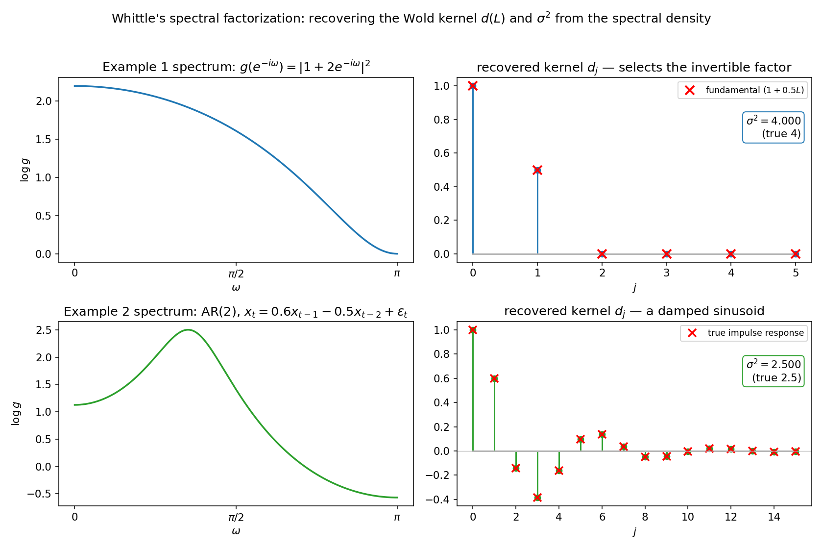
Fig. 15 Figure. Whittle’s spectral factorization recovers the fundamental Wold kernel \(d(L)\) and the innovation variance \(\sigma^2\) from the spectral density alone, by way of the cepstrum. Top: the non-invertible MA(1) spectrum \(\bigl|1 + 2e^{-i\omega}\bigr|^2\) (left); the recovered kernel (stems, right) lands on the fundamental factor \(1 + \tfrac12 L\) (red \(\times\)), with \(\sigma^2 = 4\). Bottom: an AR(2) with complex roots, whose spectrum peaks near \(\omega \approx 2\pi/9\) (left); the recovered kernel (stems, right) reproduces the autoregression’s damped-sinusoid impulse response (red \(\times\)), with \(\sigma^2 = 2.5\). Generated by code/ch13_whittle_factor.py.

The method is the computational complement to Wold’s theorem: where the theorem asserts that a fundamental \(d(L)\) and a variance \(\sigma^2\) exist, Whittle’s factorization computes them from the second moments, packaged as the spectral density, in a handful of Fourier transforms.

---

[1]

The \(a_i^n\) will be unique only if there are no linear dependencies across the \(x_{t-i}\). The projection of \(x_t\) on the space spanned by \(\,\{x_{t-1}, x_{t-2}, \ldots, x_{t-n}\}\) is unique even without that condition.

[2]

It is not necessarily true that the sequence of \(a_t^n\) settles down nicely as \(n \to \infty\), only that successive \(\hat{x}_t^n\) get closer to each other and to \(\hat{x}_t\), as \(n \to \infty\).

[3]

For a proof, see Anderson (1971, p.419).

[4]

See Wold (1938). The proof given here parallels that given by Anderson (1971). The reader familiar with Hilbert spaces is urged to read Anderson at this point.

[5]

That is, the sequence of \(\sum_{j=0}^{m} d_j \epsilon_{t-j}\) is a Cauchy sequence. In particular, for \(n > m\), \(E(\sum_{j=0}^m d_j \epsilon_{t-j} - \sum_{j=0}^n d_j \epsilon_{t-j})^2 = E(\sum_{j=m+1}^n d_j^2 \epsilon_{t-j}^2) = \sigma^2 \sum_{j=m+1}^n d_j^2\). Since \(\sum_{j=0}^{\infty} d_j^2 < \infty\), it follows that we can choose an \(m\) big enough to drive \(\sigma^2 \sum_{j=m+1}^n d_j^2\) arbitrarily close to zero.

[6]

Those linear combinations \(\sum_{j=1}^{\infty} f_j x_{t-j}\) for which \(\sum_{j=1}^{\infty} f_j^2 < \infty\), so that the variance of the sum is finite.

[7]

This is an implication of the orthogonality principle. See Anderson (1971).

[8]

For example, let \(x(t) = a \cos \lambda t + b \sin \lambda t\) where \(E a = E ab = E b = 0, \quad E a^2 = E b^2 = \sigma^2\). Then: \(Ex(t_1)x(t_2) = E\{a^2 \cos \lambda t_1 \cos \lambda t_2 + a b (\sin \lambda t_2 \cos \lambda t_1 + \cos \lambda t_2 \sin \lambda t_1) + b^2 \sin \lambda t_1 \sin \lambda t_2 \} = \sigma^2\{\cos \lambda t_1 \cos \lambda t_2 + \sin \lambda t_1 \sin \lambda t_2\}\). Since \(\cos(\alpha - \beta) = \cos \alpha \cos \beta + \sin \alpha \sin \beta\), we have \(E x(t_1) x(t_2) = \sigma^2 \cos \lambda(t_1 - t_2)\) or \(E x(t) x(t-T) = \sigma^2 \cos \lambda T\). These calculations can easily be extended to prove the assertion made in the text.

[9]

There are essentially two ways in which a process can be deterministic. One is if its spectral density consists entirely of a number of “spikes” or delta functions. A second way is if its spectral density, even though having no spikes, is zero on some interval of \(\omega\)’s of positive length, or is “too close” to zero over such an interval. Heuristically, this second possible way of being deterministic is suggested by the Kolmogorov formula for the one-step-ahead prediction error variance \(\sigma_t^2 = \exp[(2 \pi)^{-1} \int_{-\pi}^{\pi} \ln g(e^{-i \omega})d\omega]\) where \(g(e^{-i\omega})\) is the spectral density. See Whittle (1983, p. 26).