Seasonality and Approximation Errors#
Note
This section is based on Lars Peter Hansen and Thomas J. Sargent, “Seasonality and approximation errors in rational expectations models,” Journal of Econometrics 55 (1993), 21–55. We follow the paper’s Sections 2–5 and have condensed and reorganized the exposition.
The previous section, Seasonal Adjustment and Forecasting Geometric Distributed Leads, showed mechanically how an econometrician misspecifies the cross-equation restrictions when he applies the Hansen–Sargent geometric-lead formula (282) to seasonally adjusted data while agents actually forecast the unadjusted series. That analysis presumed the model was otherwise correctly specified, and it delivered a clean verdict: seasonal adjustment distorts the implied restrictions.
But that is not the end of the argument. Sims (1976) countered that a model is almost always an approximation, and that if the approximation is worst at the seasonal frequencies — where the raw data have most of their power — then an econometrician might obtain better estimates of the economically interesting parameters (of preferences and technology) by using seasonally adjusted data and giving up the pretense of fitting the seasonal. To adjudicate this claim one needs a criterion that says exactly what a misspecified maximum-likelihood estimator converges to, frequency by frequency. This section develops that criterion — a frequency-domain representation of the Kullback–Leibler information that Gaussian maximum likelihood implicitly minimizes — and uses it to compare adjusted with unadjusted data.
A covariance-stationary model of seasonality#
Let \(s(t)\) be a periodic seasonal indicator, \(s(t+p)=s(t)\), mapping calendar time into one of \(p\) seasons. To keep the process stationary rather than merely periodic, Hansen and Sargent randomize the phase: they draw, once and for all, one of the \(p\) calendar alignments of \(s\), each with probability \(1/p\). The resulting \(\{s(t)\}\) is strictly stationary and ergodic, yet deterministic — knowing it at one date reveals it at all dates — so conditioning on the whole path is the same as conditioning on \(s(t)\). Write \(E[\,\cdot \mid s(t)\,]\) for that conditional expectation.
Combine \(\{s(t)\}\) with an \((n\times 1)\) martingale difference sequence \(\{w_t\}\), \(E[w_t w_t' \mid w_{t-1},\ldots ; s] = I\), to build the periodic linear model
where \(y_t\) is the \((m\times 1)\) vector observed by the econometrician and \(\nu_{s(t)}\) is an \((m\times 1)\) vector of seasonal means. Both the moving-average kernel \(M_{s(t)}(L)\) and the mean \(\nu_{s(t)}\) are allowed to depend on the season. Because \(\{s(t)\}\) and \(\{w_t\}\) are jointly stationary and ergodic, so is \(\{y_t\}\), and a law of large numbers applies.
There are now two natural ways to form sample moments, and they converge to different limits. Averaging conditionally on the season (skip-sampling every \(p\) periods) recovers the season-specific means and autocovariances,
while averaging unconditionally recovers their season-averages,
This gap between conditional and unconditional second moments is the crux of the whole analysis: periodicity lives in the conditional moments, and an econometrician who forms ordinary (unconditional) sample moments effectively looks only at the averages (380).
To make the periodic model tractable it helps to stack \(p\) consecutive observations into a single vector, \(Y_t = [\,\bar y_{p(t-1)+1}'\ \cdots\ \bar y_{pt}'\,]'\), and likewise for the noise \(W_t\). The stacked process has period one,
with \(S_Y\) its covariance generating function (see A Mathematical Digression: Fourier and z Transforms and The Spectrum). The bridge back to the ordinary (unstacked, unconditional) covariance generating function \(s_y(z) = \sum_k z^{-k} r(-k)\) is the Tiao–Grupe formula,
Formula (382) records exactly the restrictions a periodic model imposes on second moments computed the ordinary way — and it is what lets us predict the misinterpretations of an econometrician who ignores hidden periodicity.
Three economic sources of seasonality#
Where does the periodic structure (378) come from economically? Hansen and Sargent exhibit a single linear-quadratic planning problem whose equilibrium takes the form (378) and which can generate seasonality in three distinct ways. A planner chooses \(\{c_t, k_t, i_t\}\) to maximize
subject to the technology and shock processes
with \(a_b, a_d\) scalar autoregressive operators with zeros outside the unit circle. Here \(c_t\) is consumption, \(k_t\) capital, \(i_t\) investment, \(\ell_t\) the labor used to adjust capital, and \(\{b_t\}, \{d_t\}\) are preference and endowment shocks. This is a linear-quadratic optimum-growth model (Brock–Mirman, with Ryder–Heal preferences and Lucas–Prescott adjustment costs); its solution for \(y_t = [c_t\ i_t]'\) has the form (378). The habit term is a seasonal one: it links \(c_t\) to consumption \(p\) periods earlier, \(c_{t-p\cdot j}\).
The three seasonality mechanisms correspond to which piece of the model is switched on:
(a) Exogenous seasonality. Set \(\lambda=0\) and \(\gamma_{s(t)}=\gamma\) constant, but let \(a_b(L)\) or \(a_d(L)\) put spectral peaks at the seasonal frequencies. The seasonality of the shocks is transmitted to \((c_t,i_t)\) through the decision rules. The model is time-invariant.
(b) A seasonal propagation mechanism. Keep \(\gamma_{s(t)}=\gamma\) and shocks with no seasonal peaks, but activate seasonal habit persistence, \(\lambda>0\). Preferences alone induce spectral peaks in \((c_t,i_t)\) at the seasonal frequencies. Again time-invariant.
(c) Periodic coefficients. Set \(\lambda=0\) and non-seasonal shocks, but let the productivity parameter \(\gamma_{s(t)}\) vary periodically. The equilibrium is genuinely periodic — form (378) with season-dependent \(M_{s(t)}\) — and the Tiao–Grupe fold (382) transmits seasonality to the ordinary spectral density of \(\{y_t\}\).
All three deliver spectral peaks at the seasonal frequencies in the observables; they differ in whether the peaks come from the shocks, from tastes/technology, or from hidden periodicity.
Sims’s approximation error formula#
Sims’s formula is the scalar ancestor of the criterion developed below. Let \((y_t, x_t)\) be jointly covariance stationary with means of zero, let \(b^0(L)\) be the two-sided linear least squares projection of \(y_t\) on the whole \(x\) process, and let a researcher fit \(y_t = b^1(L) x_t + u_t\) by least squares under a constrained parameterization that rules out \(b^1 = b^0\). In population, least squares picks \(b^1\) to minimize
where \(g_x\) is the spectral density of \(x\). The spectral density of the regressor weights the approximation error. A constrained \(b^1\) tracks \(b^0\) closely at frequencies where \(x\) has most of its power and departs from \(b^0\) where \(x\) has little. Exercise 33 asks for a derivation.
Three sections of this book turn on (385). The present section extends it to the multivariate, mean-augmented case and uses it to adjudicate Sims’s claim about seasonal adjustment. Money Demand in Hyperinflations: A Misspecified Regression and Sims’s Approximation Formula uses it to explain what a misspecified regression of money on inflation estimates in a hyperinflation. Lucas’s Two Illustrations of the Quantity Theory and Whiteman’s Critique uses it to explain what Lucas’s filtered scatterplots of money and prices estimate.
The approximation criterion#
Now suppose the econometrician fits an approximating model indexed by a parameter vector \(\delta\), with mean \(\mu(\delta)\) and spectral density \(G(\cdot,\delta)\) for the stacked process \(\{Y_t\}\), while the truth has mean \(\nu\) and spectral density \(F(\omega) = S_Y[\exp(-i\omega)]\). Estimating \(\delta\) by Gaussian maximum likelihood is, as Akaike (1973) and White (1982) stressed, a way of minimizing a Kullback–Leibler discrepancy. For stationary linear time series the population limit of the (misspecified) log-likelihood has a clean frequency-domain representation — an extension of (385) to the multivariate, mean-augmented case (Sims, 1972). The maximum-likelihood estimator converges almost surely to the minimizer of
where
The three terms have transparent meanings. \(A_1\) is (essentially) the log-determinant of the one-step-ahead forecast-error covariance implied by the approximating model — the “own” size of the fitted innovations. \(A_2\) is the limiting quadratic form that the likelihood builds from the data covariances, and it is where the truth \(F\) enters: it penalizes mismatch between \(G\) and \(F\), weighted by \(F\) itself. \(A_3\) penalizes errors in the mean, using the approximating zero-frequency spectral density as its metric. This is the same Whittle/Hannan spectral likelihood that drives the estimation section of Exact Linear Rational Expectations Models; here it is put to a different use. For computation one replaces the integrals by a Riemann sum over \(\omega_j = 2\pi j/N\),
exploiting conjugate symmetry to halve the terms.
Ignoring periodicity. When the approximating model treats \(\{y_t\}\) as time-invariant — using a single spectral density \(g(\cdot,\delta)\) and ignoring the periodic structure of the conditional autocovariances — the stacked density \(G\) factors through the fold (382). Because the columns of the stacking matrix are orthonormal, \(A_1\) and \(A_2\) collapse to ordinary, unstacked integrals,
where \(f(\omega)\) is the ordinary spectral density of the mean-adjusted \(\{\bar y_t\}\) and the last step uses Tiao–Grupe (382). In words: an econometrician who ignores hidden periodicity is simply matching the ordinary spectral density \(f\) with his time-invariant \(g\), paying no attention to the season-by-season conditional moments.
Adjusted versus unadjusted data#
The criterion (386) lets us pose Sims’s question precisely. Two experiments:
Unadjusted data. Criterion (386) applies as written, with the true density \(F\).
Seasonally adjusted data. Passing the data through a (two-sided, symmetric) seasonal-adjustment filter matrix \(c(L)\) replaces \(F(\omega)\) by \(F^a(\omega) = c(e^{-i\omega})\, F(\omega)\, c(e^{i\omega})'\) in \(A_2\). The ideal limiting case is a band-pass filter that deletes the seasonal frequencies outright: insert an indicator \(C(\omega)\), equal to one except at the seasonal frequencies and zero there,
(390)#\[A(\delta) = \frac{1}{2\pi}\int_{-\pi}^{\pi} C(\omega)\Big\{\log\det G(\omega,\delta) + \operatorname{trace}\!\big[G(\omega,\delta)^{-1} F(\omega)\big]\Big\}\, d\omega + [\nu-\mu(\delta)]'\, G(0,\delta)^{-1}\, [\nu-\mu(\delta)].\]
Now Sims’s argument reads directly off \(A_2\). Because \(A_2\) weights the fit by \(F(\omega)\) (or \(F^a(\omega)\)), it assigns the most weight to approximation error where the data have the most power — and for seasonal series that is precisely the seasonal frequencies, which are also where a model builder least trusts his specification. Down-weighting those frequencies by seasonal adjustment therefore diminishes the leverage that seasonal misspecification exerts on the estimates of preference and technology parameters. The point is not to estimate the seasonal autoregressions \(a_b(L), a_d(L)\) better — those get worse — but to buy better estimates of the parameters one actually cares about by sacrificing the seasonal fit.
Against this stands a countervailing efficiency loss when the model is correctly specified. The very cross-equation, cross-frequency restrictions of a rational-expectations model (cf. Some Applications to Rational Expectations Models and Exact Linear Rational Expectations Models) are most informative exactly at the high-power seasonal frequencies, so throwing those frequencies away discards overidentifying information. Whether this matters for consistency is settled by the information inequality: for each \(\omega\),
with equality if and only if \(G(\omega,\delta) = F(\omega)\). Hence if the model is correctly specified — there is a \(\delta_0\) with \(G(\cdot,\delta_0) = F\) everywhere and \(\mu(\delta_0)=\nu\) — then \(\delta_0\) minimizes the integrand frequency by frequency, so it remains a minimizer of the band-pass criterion (390) even after the seasonal frequencies are deleted. Seasonal adjustment then costs no consistency, only efficiency (and only if the model is genuinely correct at the seasonal frequencies too).
The five examples#
Hansen and Sargent solve the planning model of (383)–(384) for the equilibrium moving-average representation of \(y_t = [c_t\ i_t]'\), form its spectral density, and minimize the discretized criterion (388) numerically under each data treatment. All five examples are quarterly (\(p=4\), so the seasonal frequencies are \(\omega=\pi/2\) and \(\omega=\pi\)) and share \(\delta_k = 0.95\) and \(\beta = 1/1.05\).
Note
The spectral-density figures below are reconstructions: they are produced by solving the linear-quadratic model with the paper’s parameters (the solver is validated against its analytic Euler equation and by matching spectral-area to variance) rather than reproduced pixel-for-pixel from the 1993 originals. The endowment lag structure is read as free coefficients at lags \(1,4,5\), consistent with the parameter labels \(a_1,a_4,a_5\) in Table 1 and with the lag-4 (annual) term that generates quarterly seasonality.
Example 5.1 — a time-invariant fit to a periodic truth#
The true model is of category (c): a periodic productivity \(\gamma_{s(t)} = (0.13,\,0.1,\,0.1,\,0.08)\), no habit (\(\lambda=0\)), \(\phi_1 = 0.3\), preference shock \(a_b(L)=1-0.2L\) with \(\sigma_{w_1}=0.25\), and endowment shock \(a_d(L)=1-0.4L\) with \(\sigma_{w_2}=1\). The econometrician fits a time-invariant model (category a), ignoring the hidden periodicity, and soaks up seasonality through a restricted fifth-order endowment autoregression with free coefficients at lags \(1,4,5\): \(d'_t = a_1 d'_{t-1} + a_4 d'_{t-4} + a_5 d'_{t-5} + w_{2t}\). He estimates \(\gamma,\phi_1,a_1,a_4,a_5\); the results under the three data treatments are:
Parameter |
Seasonally unadjusted |
No means removed |
Seasonally adjusted |
Truth |
|---|---|---|---|---|
\(\gamma\) |
0.0996 |
0.1030 |
0.1025 |
\(\gamma_{s(t)}\) (avg. \(0.1025\)) |
\(\phi_1\) |
0.4132 |
0.2854 |
0.3007 |
0.3000 |
\(a_1\) |
0.931 |
0.3250 |
0.3987 |
0.4000 |
\(a_4\) |
0.4383 |
0.1598 |
\(-0.0003\) |
0.000 |
\(a_5\) |
\(-0.4298\) |
\(-0.1261\) |
\(-0.0005\) |
0.000 |
Table 1. Estimated time-invariant model when the true model is periodic (Hansen–Sargent 1993).
With unadjusted data the estimator falsely imputes seasonality to the endowment (\(a_4\approx0.44\), \(a_5\approx-0.43\)) and badly distorts the adjustment cost \(\phi_1\), straining to match power at the seasonal bands. With ideally adjusted data the spurious seasonal coefficients collapse to \(a_4,a_5\approx 0\), \(\phi_1\approx 0.30\), and \(\gamma\approx 0.1025\), the arithmetic average of the periodic \(\gamma_{s(t)}\) — excellent estimates of the economic parameters. This is Sims’s bias-reduction case. (Because periodic productivity injects most of its seasonality into the periodic means \(\nu_{s(t)}\) rather than the autocovariances, the “no means removed” column — which lets the mean term \(A_3\) act — is the worst of all, and the stochastic seasonality in this example is comparatively mild.)
Examples 5.2 and 5.5 — seasonal habit persistence#
The true model is of category (b): time-invariant with seasonal habit persistence, \(\lambda=0.8\), \(\delta_h=0.9\), \(\gamma=0.1\), \(\phi_1=0.005\), endowment \(a_d = 0.7\) (\(\sigma_{w_2}=1\)), preference shock \(a_b=0.2\) (\(\sigma_{w_1}=0.25\)). The habit term links \(c_t\) to \(c_{t-4}, c_{t-8}, \ldots\) and drives sharp spectral peaks into consumption and investment at \(\omega=\pi/2\) and \(\omega=\pi\) (Fig. 22).
Example 5.2 (correctly specified). The econometrician fits the true model, estimating \(\delta_h,\lambda,\gamma,a_1,\phi_1\). All three data treatments — unadjusted, unadjusted with seasonal means removed, and ideally adjusted (seasonal band deleted) — recover the true parameters exactly, even though \(\lambda,\delta_h\) act primarily at the seasonal frequencies. The cross-frequency restrictions pin the habit parameters down from the nonseasonal frequencies alone; this is the “no inconsistency” case of (391). In Fig. 22 the correctly specified spectrum lies exactly atop the truth.
Example 5.5 (habit omitted). The econometrician erroneously sets \(\lambda=0,\delta_h=0\) and fits an AR(1) endowment on ideally adjusted data, obtaining \(\gamma=0.1000\), \(\phi_1=0.0043\), \(a_1=0.4019\). The technology parameters \(\gamma,\phi_1\) stay near their truths, but the autoregressive parameter is far from its true value of \(0.7\), and — as the dashed curve in Fig. 22 shows — the fitted model cannot reproduce the seasonal peaks at all.
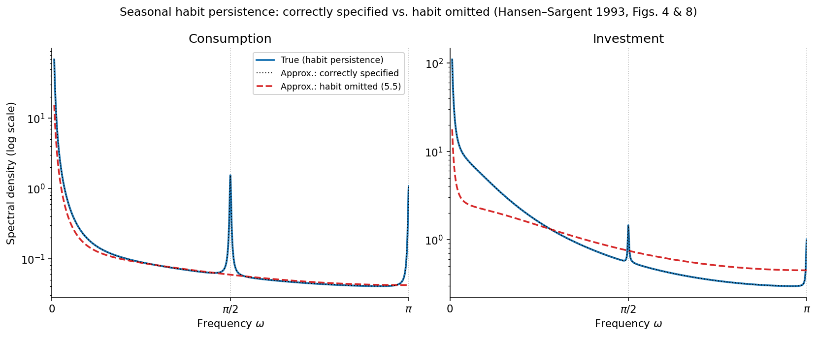
Fig. 22 Consumption and investment spectra (log scale) when the true model has seasonal habit
persistence (Example 5.2/5.5; reconstruction of Hansen–Sargent 1993, Figs. 4 and 8). The habit
term places sharp peaks at the quarterly seasonal frequencies \(\omega=\pi/2,\pi\) (dotted verticals).
The correctly specified approximating model (black dotted) lies atop the true spectrum
(blue) — every data treatment recovers the truth. The habit-omitted model (red dashed, Example
5.5) matches the technology parameters but entirely misses the seasonal peaks. Generated by
code/ch33a_fig_habit.py.#
Examples 5.3 and 5.4 — a seasonal endowment and too short an autoregression#
The true model is of category (a): time-invariant, \(\gamma=0.1\), \(\phi_1=0.3\), with a seasonal endowment \(d'_t = 0.1 d'_{t-1} + 0.5 d'_{t-4} - 0.4 d'_{t-5} + w_{2t}\) (\(\sigma_{w_2}=1\)) whose lag-4/5 terms drive seasonal peaks (most visibly near \(\omega=\pi\)) into the observables.
Example 5.3 (correctly specified). The econometrician fits the true model — using data on either \(\{c_t,i_t\}\) or \(\{c_t,d_t\}\) — and recovers all five parameters under every data treatment, again by the strength of the cross-frequency restrictions.
Example 5.4 (too short an autoregression). The econometrician imposes \(a_4=a_5=0\), fitting only a first-order endowment autoregression. He recovers \(\gamma=0.1000\), \(\phi_1=0.3011\), \(a_1=0.1631\) with adjusted data, versus \(\gamma=0.1003\), \(\phi_1=0.2964\), \(a_1=-0.2018\) with unadjusted data. The technology parameters are close either way, but the unadjusted fit is worse: it drives \(a_1\) negative in a vain effort to place power near \(\omega=\pi\), as the dash-dot curve in Fig. 23 shows.
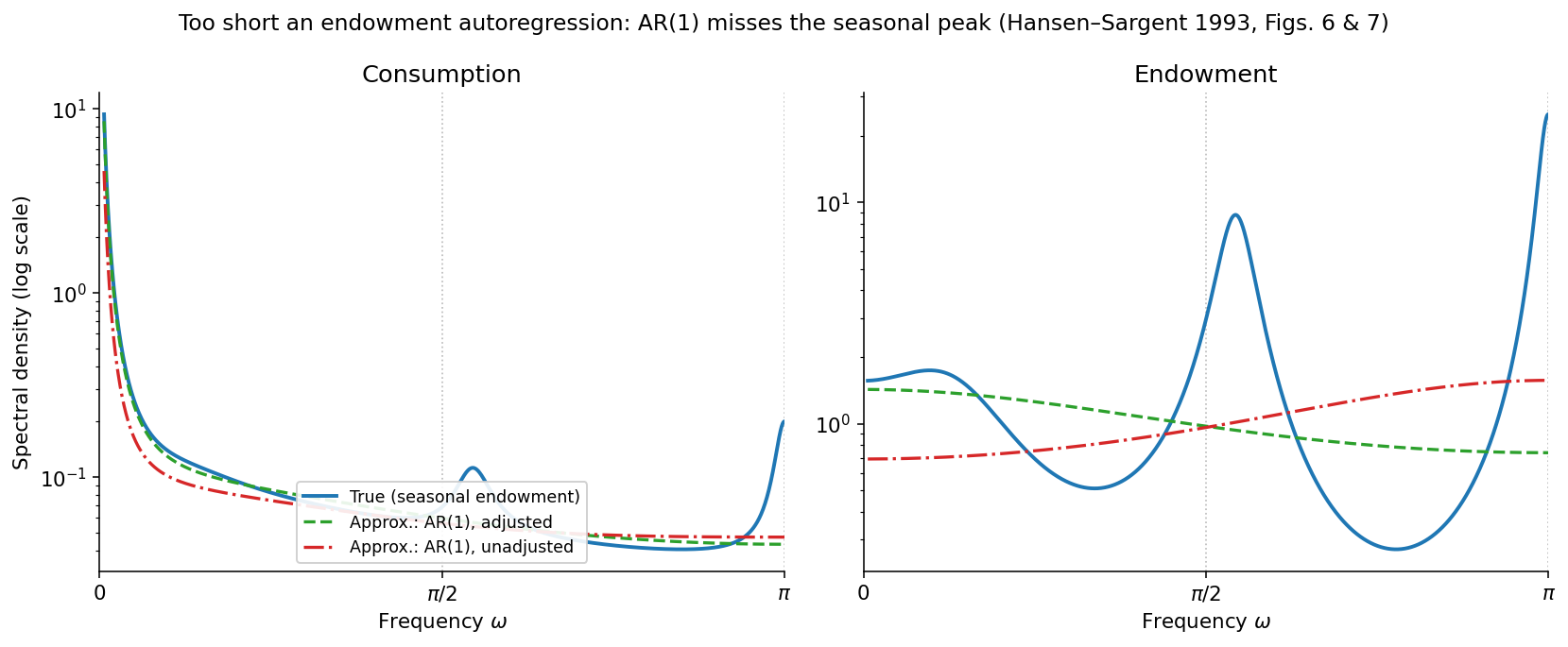
Fig. 23 Consumption and endowment spectra (log scale) when the true endowment is seasonal but the
econometrician fits a first-order autoregression (Example 5.4; reconstruction of Hansen–Sargent
1993, Figs. 6 and 7). The true endowment (blue, right panel) has pronounced seasonal structure that
neither AR(1) approximation can reproduce; the unadjusted fit (red dash-dot) tilts its spectrum
up toward \(\omega=\pi\) (a negative \(a_1\)) chasing the seasonal peak, while the adjusted fit
(green dashed) tilts down. Generated by
code/ch33a_fig_shortar.py.#
The lessons#
Taken together: when the model is misspecified at the seasonal frequencies (5.1, 5.4, 5.5), seasonally adjusted data deliver markedly better estimates of the preference and technology parameters; when the model is correctly specified (5.2, 5.3), every data treatment — including ideal adjustment that deletes the seasonal band — recovers the truth, thanks to the cross-frequency overidentifying restrictions.
These examples induce healthy skepticism toward any blanket rule of always using unadjusted data, and lend support to Sims’s recommendation — with an important asymmetry. When the model is correctly specified (in the strong sense of matching all frequencies), estimating it with seasonally adjusted data entails no inconsistency; when it is misspecified at the seasonal frequencies, seasonal adjustment can sharply reduce asymptotic bias. The caveat is that “correctly specified” must include the seasonal frequencies that adjustment then discards, so this result does not license fitting a model that implies little seasonality to data that are in fact highly seasonal.
Finally, nothing in the argument is special to seasonal frequencies. The same criterion (386) rationalizes matching a model only over a chosen band — for example, fitting a business-cycle model to Hodrick–Prescott high-pass–filtered data while distrusting the model’s low-frequency implications (compare the band definitions in Alternative Definitions of the Business Cycle). Seasonal adjustment is just one instance of deliberately down-weighting frequencies where one distrusts the model.
Exercises#
Exercise 30 (The information inequality and “no inconsistency”)
Let \(F\) and \(G\) be \((m\times m)\) Hermitian positive-definite spectral density matrices.
(a) Show that for each \(\omega\), \(\log\det G + \operatorname{trace}(G^{-1}F) \ge \log\det F + m\), with equality iff \(G = F\). Hint: let \(\lambda_1,\dots,\lambda_m>0\) be the eigenvalues of \(G^{-1}F\); the inequality reduces to \(\sum_k(\lambda_k - \log\lambda_k) \ge m\), which follows term-by-term from \(x-\log x \ge 1\) with equality iff \(x=1\).
(b) Conclude that if the approximating model is correctly specified — there is a \(\delta_0\) with \(G(\cdot,\delta_0)=F\) and \(\mu(\delta_0)=\nu\) — then \(\delta_0\) minimizes the integrand of \(A_1+A_2\) at every frequency, and hence remains a minimizer of the band-pass criterion (390) even when the seasonal frequencies are deleted by \(C(\omega)\).
(c) Explain why deleting frequencies nonetheless generically raises the asymptotic variance of the estimator, and identify the one circumstance (hint: purely seasonal, linearly deterministic measurement error) under which deletion carries no efficiency cost.
Solution to Exercise 30 (The information inequality and "no inconsistency")
(a) Because \(G\) and \(F\) are Hermitian positive definite, \(G^{-1}F\) is similar to the Hermitian positive-definite matrix \(G^{-1/2} F G^{-1/2}\), so its eigenvalues \(\lambda_1,\dots,\lambda_m\) are real and strictly positive. Then
Subtracting,
since \(x - \log x - 1 \ge 0\) for every \(x>0\) (the function is convex with its unique minimum, \(0\), at \(x=1\)). Equality holds iff every \(\lambda_k = 1\), i.e. \(G^{-1}F = I\), i.e. \(G = F\).
(b) At \(\delta_0\) we have \(G(\omega,\delta_0) = F(\omega)\) for every \(\omega\), so by part (a) the integrand \(\log\det G(\omega,\delta) + \operatorname{trace}[G(\omega,\delta)^{-1}F(\omega)]\) attains its pointwise minimum \(\log\det F(\omega) + m\) at \(\delta = \delta_0\), simultaneously at every frequency. Hence \(\delta_0\) minimizes \(A_1 + A_2\); and since \(\mu(\delta_0)=\nu\) we have \(A_3(\delta_0)=0\), its minimum, so \(\delta_0\) minimizes \(A\). Inserting the indicator \(C(\omega)\in\{0,1\}\) merely deletes some of these already-minimized terms from the integral, and the survivors are still minimized termwise at \(\delta_0\); therefore \(\delta_0\) remains a minimizer of the band-pass criterion (390). Estimation with (ideally) seasonally adjusted data is thus consistent. (Deletion can, however, introduce extra minimizers — parameter values that match \(F\) only off the seasonal band — so identification may be lost even where consistency is not.)
(c) Away from \(\delta_0\) each frequency contributes a strictly positive penalty \(\sum_k(\lambda_k(\omega) - \log\lambda_k(\omega) - 1) > 0\); these penalties are what curve the criterion around \(\delta_0\) and pin the estimator down. Deleting the seasonal frequencies discards the penalties they would contribute. Because the model’s cross-equation, cross-frequency restrictions make the seasonal-band behavior depend on the same parameters as the rest of the spectrum, this flattens the criterion precisely along the directions those restrictions constrain, inflating the asymptotic variance. The exception is a purely seasonal, linearly deterministic measurement error: being perfectly predictable from its own past, it carries no information about the structural parameters, so the seasonal frequencies were uninformative to begin with — deleting them removes contamination at no efficiency cost.
Exercise 31 (Stacking and the Tiao–Grupe fold)
Consider a scalar (\(m=1\)), period-\(p=2\) process with seasonal variances but no serial dependence: \(\bar y_t = \mu_{s(t)}\, w_t\), where \(w_t\) is unit-variance white noise and \(\mu_{s(t)}\) alternates between \(\mu_1\) and \(\mu_2\).
(a) Form the stacked process \(Y_t = [\bar y_{2t-1}\ \ \bar y_{2t}]'\), and show its moving-average operator is the constant matrix \(\bar M(L) = \operatorname{diag}(\mu_1,\mu_2)\), so that \(S_Y(z) = \operatorname{diag}(\mu_1^2,\mu_2^2)\).
(b) Using the Tiao–Grupe formula (382) with \(Q(z) = \tfrac{1}{\sqrt{2}}[\,z^{2}\ \ z\,]'\), show that the ordinary covariance generating function is the constant \(s_y(z) = \tfrac{1}{2}(\mu_1^2 + \mu_2^2)\).
(c) Conclude that \(\{\bar y_t\}\) is white with variance \(\tfrac12(\mu_1^2+\mu_2^2)\): the periodicity in the variance is invisible to the unconditional autocovariances (380), even though it is plainly present in the conditional (skip-sampled) moments (379). Relate this to why an econometrician who forms ordinary sample moments can completely miss hidden periodicity — and why, conversely, matching only \(f(\omega)\) in (389) throws away exactly the conditional information that identifies a periodic model.
Solution to Exercise 31 (Stacking and the Tiao–Grupe fold)
(a) Because \(\bar y_t = \mu_{s(t)} w_t\) has no lags, stacking two consecutive dates gives
with \(W_t = [\,w_{2t-1}\ \ w_{2t}\,]'\) and \(E W_t W_t' = I\). The moving-average operator \(\bar M(L) = \bar M\) is a constant matrix (no powers of \(L\)), so
(b) With \(p=2\) and \(m=1\), the fold (382) reads \(s_y(z) = Q(z^{-1})'\, S_Y(z^2)\, Q(z)\) with \(Q(z) = \tfrac{1}{\sqrt 2}[\,z^2\ \ z\,]'\). Since \(S_Y\) is constant, \(S_Y(z^2) = \operatorname{diag}(\mu_1^2,\mu_2^2)\), and
(c) The generating function \(s_y(z) = \tfrac12(\mu_1^2+\mu_2^2)\) is constant in \(z\), so every coefficient except the one on \(z^0\) vanishes:
(Equivalently, directly from (380): \(r(-k) = \tfrac12\sum_{t=1}^{2} c_{s(t)}(-k)\) with \(c_s(0)=\mu_s^2\) and \(c_s(k)=0\) otherwise.) Thus \(\{\bar y_t\}\) is unconditionally white with a flat spectral density — statistically indistinguishable from ordinary white noise. Yet the season-conditional variances differ, \(E[\bar y_t^2 \mid s(t)=1] = \mu_1^2 \neq \mu_2^2 = E[\bar y_t^2 \mid s(t)=2]\). An econometrician who forms ordinary (season-blind) sample moments sees only the flat spectrum and misses the periodicity entirely; only the conditional, skip-sampled moments (379) reveal it. This is exactly why matching a time-invariant \(g(\omega)\) to \(f(\omega)\) in (389) — the criterion of a model that ignores hidden periodicity — discards the season-conditional information needed to detect and identify a periodic model.
References#
Hirotugu Akaike. Information theory and an extension of the maximum likelihood principle. In B. N. Petrov and F. Csáki, editors, Second International Symposium on Information Theory. Akadémiai Kiadó, Budapest, 1973.
Lars Peter Hansen and Thomas J. Sargent. Seasonality and approximation errors in rational expectations models. Journal of Econometrics, 55(1-2):21–55, 1993.
Christopher A. Sims. The role of approximate prior restrictions in distributed lag estimation. Journal of the American Statistical Association, 67(337):169–175, 1972.
Christopher A. Sims. Seasonality in regression. Journal of the American Statistical Association, 69(347):618–626, 1974.
George C. Tiao and M. R. Grupe. Hidden periodic autoregressive-moving average models in time series data. Biometrika, 67(2):365–373, 1980.
Halbert White. Maximum likelihood estimation of misspecified models. Econometrica, 50(1):1–25, 1982.