The Spectrum

The Spectrum#

An alternative representation of the covariance generating function of \(y\) is the spectrum of the \(y\) process. Recall the covariance generating function of \(y\) defined in (158),

\[ g_y(z) = \sum_{k=-\infty}^{\infty} c_y(k)\, z^k. \]

For the process \(y_t = B(L)\epsilon_t\), we have seen that \(g_y(z) = B(z)B(z^{-1})\sigma_\epsilon^2\). If we evaluate (158) at the value \(z = e^{-i\omega}\), we have

(195)#\[g_y(e^{-i\omega}) = \sum_{k=-\infty}^{\infty} c_y(k)\, e^{-i\omega k}, \qquad -\pi < \omega < \pi.\]

Viewed as a function of angular frequency \(\omega\), \(g_y(e^{-i\omega})\) is called the spectrum of \(y\). The spectrum is the Fourier transform of the covariogram.

Inversion of the Spectrum#

As we would expect from the inversion formula (174), the spectrum is itself a kind of covariance generating function. Given an expression for \(g_y(e^{i\omega})\) it is easy to recover the covariances \(c_y(k)\) from the inversion formula (174). To motivate the inversion formula, we multiply (195) by \(e^{i\omega h}\) and integrate with respect to \(\omega\) from \(-\pi\) to \(\pi\):

(196)#\[\int_{-\pi}^{\pi} g_y(e^{-i\omega})\, e^{i\omega h}\, d\omega = \int_{-\pi}^{\pi} \sum_{k=-\infty}^{\infty} c_y(k)\, e^{i\omega(h-k)}\, d\omega = \sum_{k=-\infty}^{\infty} c_y(k) \int_{-\pi}^{\pi} e^{i\omega(h-k)}\, d\omega.\]

Now for \(h = k\), we have \(\int_{-\pi}^{\pi} e^{i\omega(h-k)} d\omega = \int_{-\pi}^{\pi} 1\, d\omega = 2\pi\). For \(h \neq k\), we have

\[ \int_{-\pi}^{\pi} e^{i\omega(h-k)}\, d\omega = \int_{-\pi}^{\pi} \cos\omega(h-k)\, d\omega + i\int_{-\pi}^{\pi} \sin\omega(h-k)\, d\omega = 0. \]

Therefore, (196) becomes

\[ \int_{-\pi}^{\pi} g_y(e^{-i\omega})\, e^{i\omega h}\, d\omega = 2\pi\, c_y(h). \]

Thus multiplying the spectrum by \(e^{i\omega h}\) and integrating from \(-\pi\) to \(\pi\) gives the \(h\)th lagged covariance times \(2\pi\). In particular, for \(h = 0\):

\[ \int_{-\pi}^{\pi} g_y(e^{-i\omega})\, d\omega = 2\pi\, c_y(0) = 2\pi \cdot \text{Var}(y), \]

so that the area under the spectrum from \(-\pi\) to \(\pi\) equals \(2\pi\) times the variance of \(y\). This fact motivates the interpretation of the spectrum as a device for decomposing the variance of a series by frequency. The portion of the variance of the series occurring between any two frequencies is given by the area under the spectrum between those two frequencies.

Properties of the Spectrum#

Notice that from (195) we have

(197)#\[g_y(e^{i\omega}) = \sum_{k=-\infty}^{\infty} c_y(k)\, e^{i\omega k} = c_y(0) + \sum_{k=1}^{\infty} c_y(k)(e^{i\omega k} + e^{-i\omega k}) = c_y(0) + 2\sum_{k=1}^{\infty} c_y(k)\cos\omega k.\]

According to (197), the spectrum is real-valued at each frequency and is obtained by multiplying the covariogram of \(y\) by a cosine function of the frequency in question. Notice also that since \(\cos x = \cos(-x)\), it follows from (197) that

\[ g_y(e^{i\omega}) = g_y(e^{-i\omega}), \]

so that the spectrum is symmetric about \(\omega = 0\). Since \(\cos(\omega + 2\pi k) = \cos(\omega)\), \(k = 0, \pm 1, \pm 2, \ldots\), it follows that the spectrum is a periodic function of \(\omega\) with period \(2\pi\). Therefore, we can confine our attention to the interval \([-\pi, \pi]\), or even \([0, \pi]\) by virtue of the symmetry.

Incidentally, the preceding calculations can be used to prove that the spectrum is always nonnegative. Suppose that the spectrum \(g_x(e^{-i\omega})\) is negative over a small band. Then choose a filter that shuts off all variance outside this band. The result is to produce a new random process that has a negative variance, a contradiction. So the spectrum must be nonnegative.

The Fundamental Filtering Formula#

We now derive a fundamental formula linking the spectrum of one covariance stationary process \(y_t\) to the spectrum of another covariance stationary process \(x_t\). We suppose that both \(\{x_t\}\) and \(\{y_t\}\) have zero mean and consider the projection equation

\[ y_t = \sum_{j=-\infty}^{\infty} b_j x_{t-j} + \epsilon_t \equiv B(L)x_t + \epsilon_t, \]

where \(E\epsilon_t x_{t-j} = 0\) for all \(j\). Here \(B(L)x_t\) is the projection of \(y_t\) on the entire \(x\) process. We then have that

\[ y_t y_{t-j} = \left(\sum_{s=-\infty}^{\infty} b_s x_{t-s}\right) \left(\sum_{r=-\infty}^{\infty} b_r x_{t-j-r}\right) + \left(\sum_{s=-\infty}^{\infty} b_s x_{t-s}\right)\epsilon_{t-j} + \left(\sum_{r=-\infty}^{\infty} b_r x_{t-j-r}\right)\epsilon_t + \epsilon_t\epsilon_{t-j}. \]

Taking expected values of both sides and applying the orthogonality conditions gives

\[ c_y(j) = E(y_t y_{t-j}) = \sum_{s=-\infty}^{\infty}\sum_{r=-\infty}^{\infty} b_s b_r c_x(j+r-s) + c_\epsilon(j). \]

The spectrum of \(y\) is defined as

(198)#\[g_y(e^{-i\omega}) = \sum_{k=-\infty}^{\infty} c_y(k)\, e^{-i\omega k} = \sum_{k,s,r} b_r b_s\, c_x(k+r-s)\, e^{-i\omega k} + g_\epsilon(e^{-i\omega}).\]

Define the index \(h = k+r-s\), so that \(k = h-r+s\). Notice that

(199)#\[e^{-i\omega k} = e^{-i\omega(h-r+s)} = e^{-i\omega h}\, e^{i\omega r}\, e^{-i\omega s}.\]

Substituting (199) into (198) gives

\[ g_y(e^{-i\omega}) = \sum_{r} b_r e^{i\omega r} \sum_{s} b_s e^{-i\omega s} \sum_{h} c_x(h) e^{-i\omega h} + g_\epsilon(e^{-i\omega}) = B(e^{i\omega})\, B(e^{-i\omega})\, g_x(e^{-i\omega}) + g_\epsilon(e^{-i\omega}), \]

or

(200)#\[g_y(e^{-i\omega}) = \left|B(e^{-i\omega})\right|^2 g_x(e^{-i\omega}) + g_\epsilon(e^{-i\omega}).\]

This is an important formula that shows how the spectrum of the “input” \(x\) is multiplied by the nonnegative real number \(|B(e^{-i\omega})|^2\) in composing the spectrum of \(y\).

Formula (200) can be used to analyze the effects of filtering, in which we start with a covariance stationary random process \(x_t\) and define a new process

(201)#\[y_t = B(L)x_t,\]

so that formula (200) applies with \(g_\epsilon(e^{-i\omega}) \equiv 0\).

Ideal Bandpass Filter#

Formula (201) motivates the interpretation of the spectrum as decomposing the variance of \(y\) by frequency. Suppose we could choose \(B(e^{-i\omega})\) so that

(202)#\[\begin{split}B(e^{-i\omega}) = \begin{cases} 1 & \omega \in [a,b] \cup [-b,-a], \quad 0 < a < b < \pi, \\ 0 & \text{otherwise.} \end{cases}\end{split}\]

A filter obeying (202) shuts off all the spectral power for frequencies not in the region \([a,b]\) or \([-b,-a]\). To determine a set of \(b_j\) that satisfies (202), we use the inversion formula:

(203)#\[b_j = \frac{1}{2\pi}\int_{-\pi}^{\pi} B(e^{-i\omega})\, e^{+i\omega j}\, d\omega = \frac{1}{2\pi}\int_{a}^{b}(e^{i\omega j} + e^{-i\omega j})\, d\omega = \frac{1}{\pi}\left(\frac{\sin jb - \sin ja}{j}\right), \qquad j \neq 0,\]

Note that \(b_j = b_{-j}\). With the \(b_j\) chosen in this way, the \(y\) process defined by \(y_t = \sum_j b_j x_{t-j}\) has all of its variance occurring in the frequency bands \(\omega \in [a,b]\), \(\omega \in [-b,-a]\). The variance of \(y\) is given by

\[ \frac{1}{2\pi}\int_{-\pi}^{\pi} g_y(e^{-i\omega})\, d\omega = \frac{1}{2\pi}\int_{-b}^{-a} g_x(e^{-i\omega})\, d\omega + \frac{1}{2\pi}\int_{a}^{b} g_x(e^{-i\omega})\, d\omega. \]

In this sense \(g_x(e^{-i\omega})\) gives a decomposition of the variance of \(x\) by frequency, the variance occurring over a given frequency band being found by integrating the spectrum over that band and dividing it by \(2\pi\).

As we shall show presently, the decomposition of the variance of \(x\) by frequency that is reflected in the spectrum is one in which components at different frequencies can be regarded as orthogonal. More precisely, two components formed by applying two filters like (202) that let through power over disjoint frequency bands are mutually orthogonal at all lags.

Spectra of Simple Processes#

White noise (\(y_t = \epsilon_t\), \(c_y(0) = \sigma_\epsilon^2\), \(c_y(h) = 0\) for \(h \neq 0\)): The covariance generating function is simply \(g_y(z) = \sigma_\epsilon^2\), so that the spectrum is

\[ g_y(e^{-i\omega}) = \sigma_\epsilon^2, \qquad -\pi \leq \omega \leq \pi. \]

The spectrum is flat, and equals \(\sigma_\epsilon^2\) at each frequency. So white noise has a flat spectrum, indicating that all frequencies between \(-\pi\) and \(\pi\) are equally important in accounting for its variance.

First-order AR (\(y_t = (1/(1-\lambda L))\epsilon_t\), \(-1 < \lambda < 1\)): The covariance generating function is \(g_y(z) = (1/(1-\lambda z))(1/(1-\lambda z^{-1}))\sigma_\epsilon^2\), so the spectrum is

\[ g_y(e^{-i\omega}) = \left(\frac{1}{1-\lambda e^{-i\omega}}\right)\!\left(\frac{1}{1-\lambda e^{i\omega}}\right)\sigma_\epsilon^2 = \frac{\sigma_\epsilon^2}{1 - 2\lambda\cos\omega + \lambda^2}. \]

Notice that

\[ \frac{dg_y(e^{-i\omega})}{d\omega} = -(1-2\lambda\cos\omega+\lambda^2)^{-2}(2\lambda\sin\omega)\,\sigma_\epsilon^2. \]

The first term in parentheses is positive. Since \(\sin\omega > 0\) for \(0 < \omega < \pi\), the second term is negative on \((0,\pi)\) if \(\lambda < 0\) and positive on \((0,\pi)\) if \(\lambda > 0\). Therefore:

If \(\lambda > 0\): spectrum decreases on \((0,\pi)\); low frequencies are relatively important in composing the variance.
If \(\lambda < 0\): spectrum increases on \((0,\pi)\); high frequencies are the more important.

It is easy to verify that the higher in absolute value is \(\lambda\), the steeper is the spectrum. Notice that the first-order process can have a peak in its spectrum only at \(\omega = 0\) or \(\omega = \pm\pi\). A peak at \(\omega = \pi\) corresponds to a periodicity of \(2\pi/\omega = 2\pi/\pi = 2\) periods. A peak at \(\omega = 0\) corresponds to a cycle with “infinite” periodicity, which is unobservable and hence not a cycle at all.

With quarterly data, a business cycle corresponds to a peak in the spectrum at a periodicity of about 12 quarters. A first-order process is capable of having a peak only at two quarters or at “infinite” quarters, and so is not consistent with a business cycle in the sense of a peak in the spectrum at about twelve quarters. As we saw above, a first-order process cannot possess a covariogram with a periodicity other than two periods, and so with quarterly data cannot deliver a business cycle in the sense of an oscillatory covariogram.

Second-order AR (\(y_t = (1-t_1L-t_2L^2)^{-1}\epsilon_t\), \(\epsilon_t\) white noise): The covariance generating function is

\[ g_y(z) = \left(\frac{1}{1-t_1z-t_2z^2}\right)\!\left(\frac{1}{1-t_1z^{-1}-t_2z^{-2}}\right)\sigma_\epsilon^2. \]

Therefore the spectrum is

\[ g_y(e^{-i\omega}) = \frac{\sigma_\epsilon^2} {1 + t_1^2 + t_2^2 - 2t_1(1-t_2)\cos\omega - 2t_2\cos 2\omega} \equiv \frac{\sigma_\epsilon^2}{h(\omega)}. \]

Differentiating with respect to \(\omega\):

\[ \frac{dg_y(e^{-i\omega})}{d\omega} = -\sigma_\epsilon^2 h(\omega)^{-2} (2\sin\omega)\bigl[t_1(1-t_2) + 4t_2\cos\omega\bigr]. \]

We know that \(h(\omega)^2 > 0\). For the above derivative to be zero at an \(\omega\) belonging to \((0, \pi)\), we must have the term in brackets equal zero:

(204)#\[t_1(1-t_2) + 4t_2\cos\omega = 0 \qquad\text{or}\qquad \cos\omega = \frac{-t_1(1-t_2)}{4t_2},\]

so that

(205)#\[\omega^* = \cos^{-1}\!\left(\frac{-t_1(1-t_2)}{4t_2}\right).\]

Equation (205) can be satisfied only if

(206)#\[\left|\frac{-t_1(1-t_2)}{4t_2}\right| < 1,\]

since \(|\cos x| \leq 1\) for all \(x\). By inspecting the second derivative of \(g_y(e^{-i\omega})\) with respect to \(\omega\), it can be verified that at the \(\omega\) given by (205) there is a peak in the spectrum if \(t_2 < 0\) and a trough if \(t_2 > 0\). Condition (206) is slightly more restrictive than the condition that roots of the deterministic difference equation be complex so that the covariogram displays oscillations. Let us write (206) as

(207)#\[-1 < -t_1(1-t_2)/4t_2 < 1.\]

The boundaries of the region (207) are

(208)#\[-t_1(1-t_2) = 4t_2\]

and

(209)#\[-t_1(1-t_2) = -4t_2.\]

The points \((t_1, t_2) = (0,0)\) appear on both boundaries, while \((t_1, t_2) = (2,-1)\) appears on (208) and \((t_1, t_2) = (-2,-1)\) appears on (209). Differentiating (208) implicitly with respect to \(t_1\) gives \(dt_2/dt_1 = (t_2-1)/(4-t_1)\), so that along (208), \(dt_2/dt_1|_{t_1=t_2=0} = -1/4\) and \(dt_2/dt_1|_{t_1=2,t_2=-1} = -1\). Differentiating (209) with respect to \(t_1\) gives \(dt_2/dt_1 = (1-t_2)/(4+t_1)\), so that along (209), \(dt_2/dt_1|_{t_1=t_2=0} = 1/4\) and \(dt_2/dt_1|_{t_1=-2,t_2=-1} = 1\).

Such calculations show that the boundaries of region (207) are as depicted in Figure 2. To be in region (207) with \(t_2 < 0\) (the case in which the stationary point is a spectral peak rather than a trough) implies that the roots of the difference equation are complex. However, complex roots do not imply that (207) is satisfied. Consequently, the conditions for an oscillatory covariogram are not quite equivalent with those for a spectral peak.

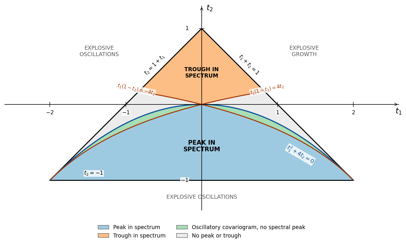
../_images/fig2_spectral_peak_region.png — Fig. 7 **Figure 2.** Parameter regions for the AR(2) process \(Y_t = t_1 Y_{t-1} + t_2 Y_{t-2} + \epsilon_t\) in the \((t_1, t_2)\) plane. The stationarity triangle is bounded by \(t_1 + t_2 = 1\), \(t_2 = 1 + t_1\), and \(t_2 = -1\). The parabola \(t_1^2 + 4t_2 = 0\) separates real roots (above) from complex roots (below). Within region (207), the spectrum has a **peak** (when \(t_2 < 0\)) or a **trough** (when \(t_2 > 0\)). The green “wings” mark the subtle case of an oscillatory covariogram with no spectral peak. After Jenkins and Watts (1969, p. 229); an extension of the QuantEcon Samuelson model stability diagram. Generated by `code/fig2_spectral_peak_region.py`.#

To illustrate the ability of low-order stochastic difference equations to generate “realistic” data, Figures 1a and 1b show simulations of first- and second-order stochastic difference equations, while figure 1c shows the solution of the deterministic part of the same second-order difference equation with initial conditions \(y_0 = y_1 = 1\). Notice that even the first-order stochastic difference equation

\[ y_t = 0.9\, y_{t-1} + \epsilon_t, \]

\(\epsilon_t\) a serially uncorrelated random term, appears to generate roughly alternating periods of boom and bust. This illustrates how stochastic difference equations can generate processes that “look like” they have business cycles even if their spectra do not have peaks on \((0, \pi)\) and even if their covariograms do not oscillate.

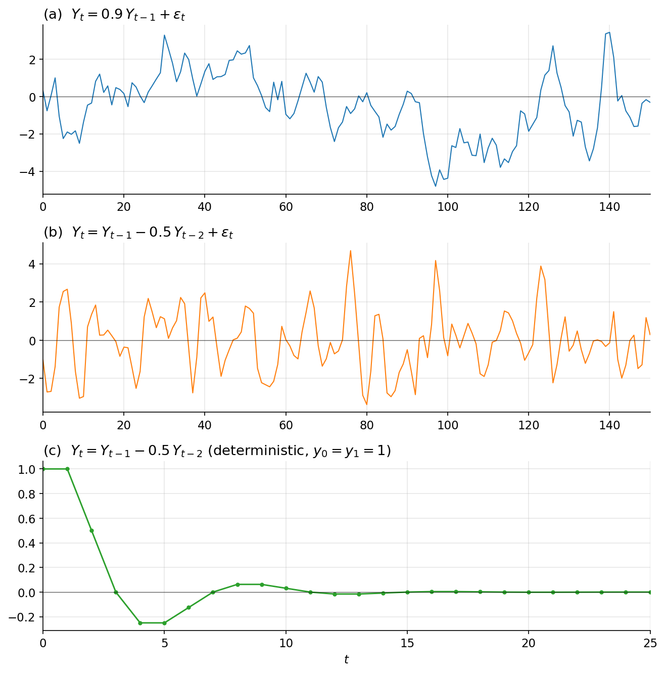
../_images/fig1_ar_realizations.png — Fig. 8 **Figure 1.** *(a)* Realization of a first-order AR process. *(b)* Realization of a second-order AR process with complex roots. *(c)* Deterministic part of the same second-order process with \(y_0 = y_1 = 1\). Generated by `code/fig1_ar_realizations.py`.#