Fourier Transform Pairs and the Uncertainty Principle

Note

Like the digression of A Mathematical Digression: Fourier and z Transforms, this short chapter develops a general property of Fourier-transform pairs and may be skipped on a first reading. It makes precise a trade-off — between concentration in time and concentration in frequency — that recurs informally throughout the book, most explicitly in the choice of filter bandwidth for complex demodulation in Complex Demodulation and of lag windows for spectral estimation in The Spectrum.

The Riesz–Fischer theorem of A Mathematical Digression: Fourier and z Transforms puts a square-summable sequence \(\{c_k\} \in l_2(-\infty,\infty)\) into one-to-one correspondence with its Fourier transform

(182)\[f(\omega) = \sum_{k=-\infty}^{\infty} c_k\, e^{-i\omega k}, \qquad \omega \in [-\pi,\pi],\]

with the inversion formula (174) recovering \(\{c_k\}\) from \(f\). The sequence and its transform are two representations of one object: a time-domain view \(\{c_k\}\) indexed by the integer \(k\), and a frequency-domain view \(f(\omega)\) indexed by \(\omega\) on the circle \([-\pi,\pi]\). The uncertainty principle is the statement that these two views cannot both be sharply localized: the more concentrated a sequence is in time, the more spread out its transform must be in frequency, and conversely.

The time–frequency duality

A few transform pairs make the duality visible.

• A single spike \(c_k = \delta_{k0}\) (one nonzero term) has the perfectly flat transform \(f(\omega) \equiv 1\). Maximal concentration in time goes with maximal spreading in frequency.

• A rectangular window \(c_k = 1\) for \(|k| \le m\) and \(0\) otherwise has, by summing the geometric series, the Dirichlet transform

  (183)\[f(\omega) = \sum_{k=-m}^{m} e^{-i\omega k} = \frac{\sin\!\big((2m+1)\omega/2\big)}{\sin(\omega/2)},\]

  whose central lobe has width of order \(2\pi/(2m+1)\). Widening the window in time (larger \(m\)) narrows its transform in frequency. This is the very filter, and the very trade-off, behind the low-pass operator \(W(L)\) of Complex Demodulation: a longer moving average resolves a narrower frequency band.

• A two-sided geometric sequence \(c_k = \lambda^{|k|}\) with \(|\lambda| < 1\) has the transform (a Poisson kernel)

  (184)\[f(\omega) = \sum_{k=-\infty}^{\infty} \lambda^{|k|} e^{-i\omega k} = \frac{1-\lambda^2}{1 - 2\lambda\cos\omega + \lambda^2},\]

  the shape of a first-order autoregressive spectrum, peaked at \(\omega = 0\) with a width of order \(1-\lambda\). As \(\lambda \uparrow 1\) the sequence decays ever more slowly (it spreads out in time) while its transform concentrates ever more sharply at the origin. The single parameter \(\lambda\) controls both the persistence in time and the bandwidth in frequency, and it cannot make both small at once.

These are instances of one inequality, which we now state quantitatively.

Making “spread” precise

Assume \(\{c_k\} \in l_2\) and, to avoid trivialities, \(c \neq 0\). Its energy is

(185)\[E = \sum_{k=-\infty}^{\infty} |c_k|^2 = \frac{1}{2\pi}\int_{-\pi}^{\pi} |f(\omega)|^2\, d\omega,\]

the two expressions being equal by Parseval’s relation. Equation (185) lets us treat the normalized \(|c_k|^2/E\) as a probability distribution over the time index \(k\), and \(|f(\omega)|^2/E\) as a probability density over frequency \(\omega\). Their means and dispersions are

(186)\[\bar k = \frac{1}{E}\sum_k k\,|c_k|^2, \qquad \Delta_t^2 = \frac{1}{E}\sum_k (k-\bar k)^2\,|c_k|^2,\]

(187)\[\bar\omega = \frac{1}{2\pi E}\int_{-\pi}^{\pi}\!\omega\,|f(\omega)|^2 d\omega, \qquad \Delta_\omega^2 = \frac{1}{2\pi E}\int_{-\pi}^{\pi}\!(\omega-\bar\omega)^2\,|f(\omega)|^2 d\omega .\]

\(\Delta_t\) is the time dispersion (the effective duration) and \(\Delta_\omega\) the frequency dispersion (the effective bandwidth). Two simplifications cost nothing. Shifting the sequence, \(c_k \mapsto c_{k-k_0}\), multiplies \(f\) by \(e^{-i\omega k_0}\) and leaves both dispersions unchanged, so we may set \(\bar k = 0\). Modulating the sequence, \(c_k \mapsto c_k e^{i\omega_0 k}\), translates \(f(\omega) \mapsto f(\omega-\omega_0)\) and again preserves the dispersions, so we may set \(\bar\omega = 0\). Assume both from now on.

The uncertainty principle

The link between the two domains is a single fact about the transform pair: differentiating the transform in frequency corresponds to multiplying the sequence by the time index. Differentiating (182) term by term,

(188)\[f'(\omega) = \sum_k (-i k)\, c_k\, e^{-i\omega k},\]

so \(f'\) is the Fourier transform of the sequence \(\{-i k\, c_k\}\). Applying Parseval (185) to that sequence gives the identity

(189)\[\frac{1}{2\pi}\int_{-\pi}^{\pi}|f'(\omega)|^2\,d\omega = \sum_k k^2\,|c_k|^2 = E\,\Delta_t^2 ,\]

the effective duration measured in the frequency domain. With \(\langle g,h\rangle = \frac{1}{2\pi}\int_{-\pi}^{\pi}\bar g\,h\,d\omega\) we have \(E\,\Delta_t^2 = \|f'\|^2\) and \(E\,\Delta_\omega^2 = \|\omega f\|^2\), so by the Cauchy–Schwarz inequality

(190)\[E\,\Delta_t\,\Delta_\omega = \|f'\|\,\|\omega f\| \;\ge\; \big|\langle \omega f,\, f'\rangle\big| \;\ge\; \big|\operatorname{Re}\langle \omega f,\, f'\rangle\big| .\]

Evaluate the real part using \(\operatorname{Re}(\bar f f') = \tfrac12(|f|^2)'\) and one integration by parts:

\[ \operatorname{Re}\langle \omega f, f'\rangle = \frac{1}{2\pi}\int_{-\pi}^{\pi}\!\omega\,\tfrac12\big(|f|^2\big)'\,d\omega = \frac{1}{2\pi}\Big\{\Big[\tfrac{\omega}{2}|f(\omega)|^2\Big]_{-\pi}^{\pi} - \tfrac12\int_{-\pi}^{\pi}\!|f|^2\,d\omega\Big\}. \]

Because \(f\) is \(2\pi\)-periodic, \(f(\pi) = f(-\pi)\), so the boundary term is \(\frac{1}{2\pi}\cdot\frac{\pi}{2}\big(|f(\pi)|^2+|f(-\pi)|^2\big) = \tfrac12|f(\pi)|^2\), while the integral is \(\tfrac12\cdot 2\pi E\). Hence \(\operatorname{Re}\langle \omega f,f'\rangle = \tfrac12\big(|f(\pi)|^2 - E\big)\), and substituting into (190) and dividing by \(E\) gives the discrete-time uncertainty principle:

(191)\[\boxed{\;\Delta_t\,\Delta_\omega \;\ge\; \frac{1}{2}\left(1 - \frac{|f(\pi)|^2}{E}\right)\;}\]

where

(192)\[\frac{|f(\pi)|^2}{E} = \frac{\big|\sum_k (-1)^k c_k\big|^2}{\sum_k |c_k|^2}\]

is the fraction of the sequence’s energy that its transform places at the Nyquist frequency \(\omega = \pm\pi\). When the sequence carries no power at \(\pm\pi\) — that is, when \(f(\pm\pi) = \sum_k(-1)^k c_k = 0\) — the correction vanishes and we recover the textbook Heisenberg bound

(193)\[\Delta_t\,\Delta_\omega \;\ge\; \frac{1}{2}.\]

The boundary term in (191) is the price of frequency living on a circle. The variable \(\omega\) jumps from \(+\pi\) back to \(-\pi\), so charging energy at \(\pm\pi\) with the dispersion \(\pi^2\) overstates how “spread” that energy really is; for sequences whose power sits away from the Nyquist frequency the correction is negligible and (193) holds to all intents. (The continuous-time transform on the whole real line has no such boundary, and the bound is exactly \(\Delta_t\Delta_\omega \ge \tfrac12\) there.)

Minimum-uncertainty sequences

Equality in (190) requires, from the Cauchy–Schwarz step, that \(f'(\omega) = -\beta\, \omega\, f(\omega)\) for some constant \(\beta > 0\). Solving this differential equation gives

(194)\[f(\omega) \propto e^{-\beta \omega^2/2},\]

a Gaussian in frequency, whose inverse transform (174) is (up to the periodic wrap-around at \(\pm\pi\)) a Gaussian sequence \(c_k \propto e^{-k^2/(2\beta)}\). Gaussian sequences are therefore the minimum-uncertainty signals — they make the duration–bandwidth product as small as it can be. They also carry essentially no Nyquist power, so the correction in (191) is negligible and they attain the clean bound \(\tfrac12\).

The figure confirms this. Panels (a) and (b) show three Gaussian sequences of increasing width and their transforms: as the sequence widens in time its transform narrows in frequency, the area of each staying fixed by Parseval. Panel (c) plots the product \(\Delta_t\,\Delta_\omega\) against the duration \(\Delta_t\) for the Gaussian family and for the rectangular windows of the preceding section. The Gaussians lie exactly on the floor \(\Delta_t\Delta_\omega = \tfrac12\) for every width; the rectangular windows — whose abrupt edges throw power into slowly decaying frequency side lobes — sit far above it (\(1.59\) at half-width \(m=5\), \(3.08\) at \(m=20\)). Concentration in time buys spreading in frequency, and the best one can do is the Gaussian compromise.

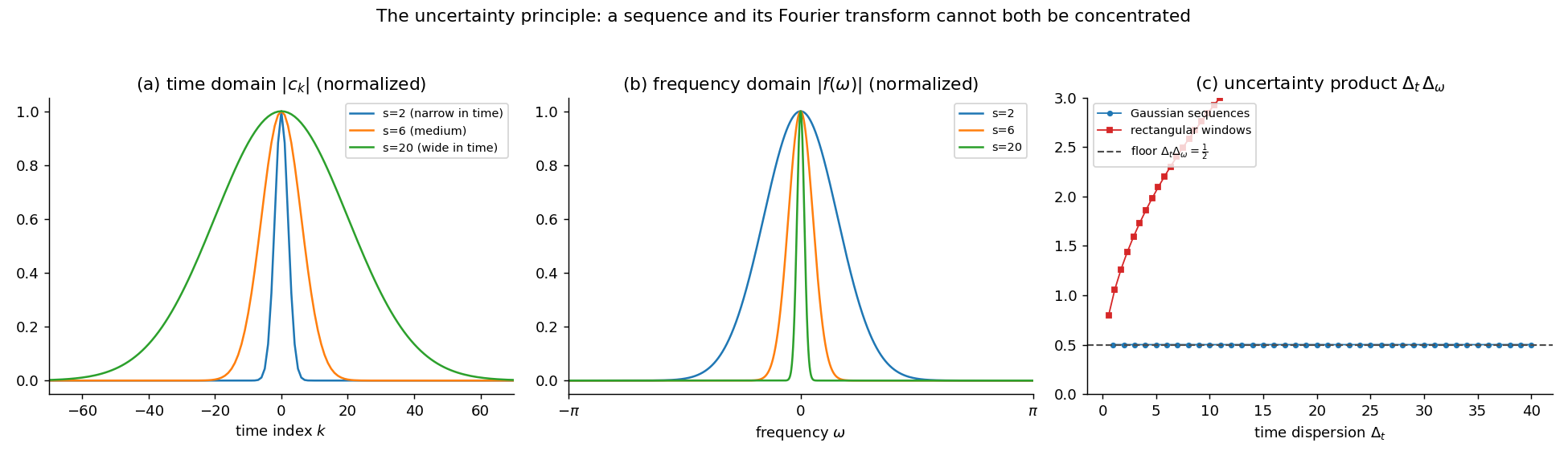
Fig. 6 Figure. The uncertainty principle for discrete-time Fourier-transform pairs. (a) Three Gaussian sequences \(c_k = e^{-k^2/2s^2}\), narrow to wide in time. (b) Their transforms \(f(\omega)\), wide to narrow in frequency — the duality. (c) The duration–bandwidth product \(\Delta_t\,\Delta_\omega\) versus \(\Delta_t\): Gaussian sequences sit exactly on the floor \(\tfrac12\) (193), while rectangular windows lie well above it. Generated by code/ch05a_uncertainty.py.

Note

The duration–bandwidth inequality (191) is the signal-processing counterpart of the Heisenberg principle of quantum mechanics, where \(|c_k|^2\) and \(|f(\omega)|^2\) play the roles of the position and momentum densities and the operators “multiply by \(k\)” and “differentiate in \(\omega\)” stand in for position and momentum. Other, sharper “versions” of the principle fix different notions of concentration: the Donoho–Stark support inequality bounds the numbers \(n_t, n_\omega\) of nonzero time and frequency samples of a length-\(N\) discrete Fourier transform by \(n_t\, n_\omega \ge N\), and there are entropic forms as well. We use the variance form because it speaks directly to the durations and bandwidths of the filters and windows used elsewhere in the book.

Why it matters here

The inequality is not a curiosity; it sets a hard limit on what time-series filtering can do. A filter that isolates a narrow band of frequencies (small \(\Delta_\omega\)) must necessarily be long in time (large \(\Delta_t\)): there is no short filter with a sharp frequency cutoff. This is exactly why the low-pass filter \(W(L)\) in complex demodulation (Complex Demodulation) faces a trade-off between frequency resolution and the number of usable observations at the ends of the sample, and why a spectral estimate (The Spectrum) cannot simultaneously have fine frequency resolution and low variance from a fixed-length record. A finite-duration sequence has a transform that is real-analytic and so cannot vanish on any interval of frequencies; a strictly band-limited sequence cannot have finite duration. The uncertainty principle is the precise form of the intuition that one buys resolution in one domain only by spending it in the other.

Exercise

Exercise 25 (The duration–bandwidth product)

1. Reproduce the floor. For the Gaussian sequence \(c_k = e^{-k^2/2s^2}\) on a long grid \(|k|\le K\), compute \(\Delta_t\) from (186) and \(\Delta_\omega\) from (187) (evaluate \(f(\omega)\) on a dense grid and integrate numerically). Verify that \(\Delta_t\,\Delta_\omega \approx \tfrac12\) for a range of \(s\), and that the Nyquist fraction (192) is negligible. Then repeat for the rectangular window \(c_k = \mathbf 1\{|k|\le m\}\) and confirm the product exceeds \(\tfrac12\), growing with \(m\).

2. An analytic case. For the two-sided geometric sequence \(c_k = \lambda^{|k|}\), sum the series to show

   \[E = \frac{1+\lambda^2}{1-\lambda^2}, \qquad \Delta_t^2 = \frac{1}{E}\sum_k k^2 \lambda^{2|k|} = \frac{2\lambda^2}{(1-\lambda^2)^2},\]

   so the duration \(\Delta_t \to \infty\) as \(\lambda \uparrow 1\). Compute \(\Delta_\omega\) numerically from the Poisson-kernel transform (184) and confirm (191). Show also that this sequence does place power at the Nyquist frequency, \(f(\pi)/\sqrt{E}\neq 0\) — using \(\sum_k(-1)^k\lambda^{|k|} = (1-\lambda)/(1+\lambda)\) — so that the relevant bound is the corrected (191), not the bare \(\tfrac12\).

3. The filter trade-off. Take the length-\((2m+1)\) moving average \(W(L)\) of Complex Demodulation and show, from the Dirichlet transform, that doubling \(m\) roughly halves the bandwidth \(\Delta_\omega\) while doubling the duration \(\Delta_t\) — the product staying fixed. Explain in one sentence what this implies for the number of observations lost at each end of a demodulated series when one demands finer frequency resolution.

4. Harder. Construct a “high-pass” sequence with most of its energy near the Nyquist frequency (e.g. \(c_k = (-1)^k e^{-k^2/2s^2}\)) and show numerically that the bare bound \(\tfrac12\) is violated while the corrected bound (191) is not. Explain how the modulation \(c_k \mapsto (-1)^k c_k\) moves energy to \(\omega = \pm\pi\) and why the circular nature of frequency makes the bare bound fail there.

References

[UPDS89]

David L. Donoho and Philip B. Stark. Uncertainty principles and signal recovery. SIAM Journal on Applied Mathematics, 49(3):906–931, 1989.

[UPFS97]

Gerald B. Folland and Alladi Sitaram. The uncertainty principle: a mathematical survey. Journal of Fourier Analysis and Applications, 3(3):207–238, 1997.

[UPGab46]

Dennis Gabor. Theory of communication. Journal of the Institution of Electrical Engineers, 93(3):429–457, 1946.

[UPSle83]

David Slepian. Some comments on fourier analysis, uncertainty and modeling. SIAM Review, 25(3):379–393, 1983.