Alternative Definitions of the Business Cycle

We have already encountered two definitions of a cycle in a single series that is governed by a stochastic difference equation. According to the first definition, a variable possesses a cycle of a given frequency if its covariogram displays damped oscillations of that frequency, which is equivalent with the condition that the nonstochastic part of the difference equation has a pair of complex roots with argument (\(\theta\) in the polar form of the root \(r e^{i\theta}\)) equal to the frequency in question. A single series is said to contain a business cycle if the cycle in question has periodicity of from about two to four years (NBER minor cycles) or about eight years (NBER major cycles).

A second definition of a cycle in a single series is the occurrence of a peak in the spectral density of a series. As we have seen, this definition is not equivalent with the previous one, but usually leads to a definition of the cycle close to the first one.

It is probably correct however that neither one of these definitions is what underlies the concept of the business cycle that most experts have in mind. In fact, most economic aggregates have spectral densities that do not display pronounced peaks at the range of frequencies associated with the business cycle. The peaks that do occur in this band of frequencies tend to be wide and of modest height. The dominant feature of the spectrum of most economic time series is that it generally decreases drastically as frequency increases, with most of the power in the low frequency, high periodicity bands. This shape was dubbed by Granger (1966) the “typical spectral shape” of an economic variable.

Figure 5 contains a record of quarterly U.S. time series for seven series over the period 1947 to the present (Sargent’s original covered 1947–1975). For each variable, the left panel plots the realization of the time series, while the right panel records an estimate of the spectral density. We record these panels side by side partly in order to give the reader some practice in “reading” spectral densities, i.e., in picturing the kind of time series realizations that are typically associated with various spectral shapes. For example, Granger’s concept of a “typical spectral shape” is illustrated by the logarithms of the spectral densities of real GNP, the unemployment rate, the real wage, the Baa rate, and output per man-hour in Figure 5. The generally downward sweeping spectrum is characteristic of a covariogram that is dominated by high, positive, low-order serial correlation. Notice that the inflation rate and change in the real money supply do not display the typical spectral shape, a characteristic that might have been anticipated from our study of the effects of applying the first difference filter \(1-L\). All of the series except the unemployment rate, which has been seasonally adjusted, display spectral peaks in the vicinity of four and two quarters, which is symptomatic of a seasonal pattern of serial correlation. “Seasonal adjustment” is a process of operating on a series with a filter \(h(L)\) that is designed to diminish the seasonal frequencies near four and two quarters, while leaving the remaining frequencies as unaffected as possible. Notice how this procedure has “succeeded” for the unemployment rate and produced dips in the spectrum near four and two quarters (see Exercise 34). Notice how real GNP has no spectral peak in the business cycle range, while output per man-hour and the unemployment rate have only very modest peaks, this despite the fact that the sample paths of all three reflect “the business cycle.” As mentioned earlier, the fact that a spectrum does not display a peak at the business cycle frequencies should not be taken to mean that the series did not experience any fluctuations associated with the business cycle. On the contrary, as Figure 1a indicated, a series could very well seem to move in sympathy with general business conditions, say as identified by the NBER, and yet have no spectral peak on the open interval \((0, \pi)\). This example cautions the reader against interpreting the lack of a peak in the spectrum at the business cycle frequencies as indicating the absence of any business cycle in the series.

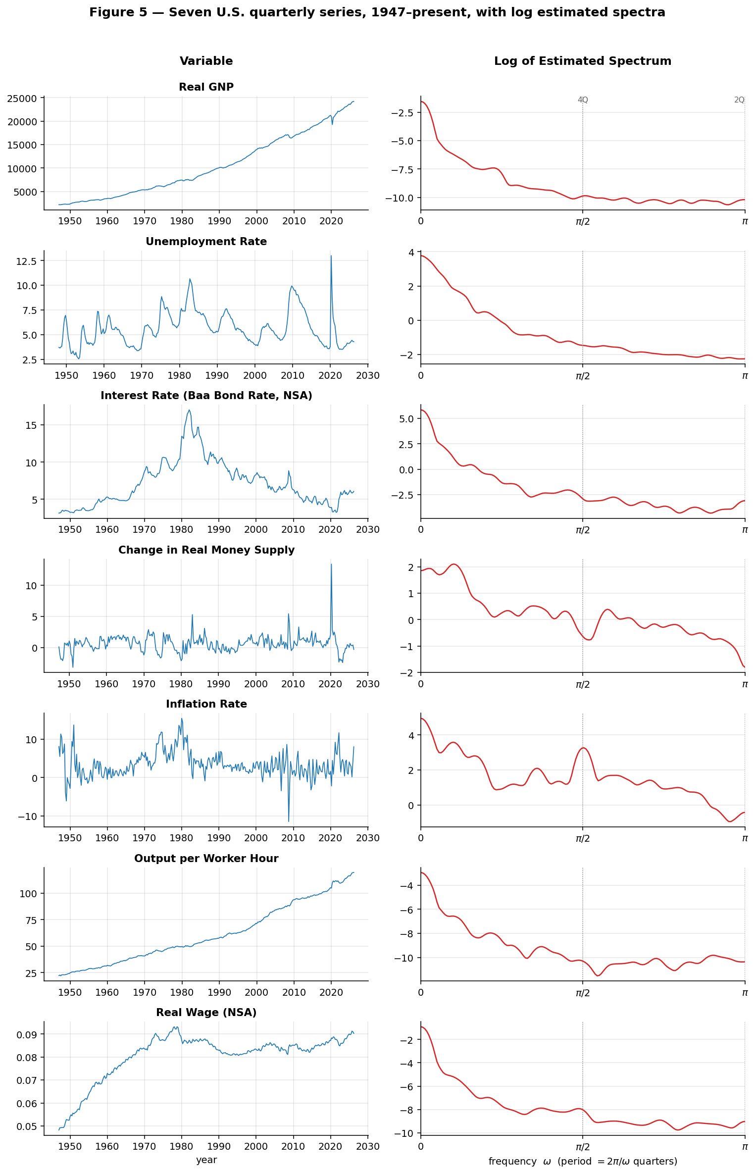
Fig. 13 Figure 5. Seven U.S. quarterly macroeconomic series, 1947–present (a modernized extension of Sargent’s original 1947–1975 figure). Left: the realized series; right: the log of an estimated spectral density (a smoothed periodogram of the linearly detrended series, in the spirit of the QuantEcon spectral estimation lecture). Note Granger’s “typical spectral shape” — the steep low-to-high frequency decline — in real GNP, the unemployment rate, the Baa rate, output per hour, and the real wage; the inflation rate and the change in real money supply depart from it. Dotted lines mark the seasonal frequencies \(\omega = \pi/2\) (4-quarter) and \(\omega = \pi\) (2-quarter). The 2020 COVID shock is retained (e.g. the unemployment spike). Data: FRED; the money supply is spliced from the NBER macrohistory series M1444CUSM027SNBR (1947–1958) onto M2SL (1959–present). Generated by code/fig5_business_cycle_series.py.

What the preceding example does indicate is that our two preceding tentative possible definitions of the business cycle are deficient. The following definition seems to capture what experts refer to as the business cycle: the business cycle is the phenomenon of a number of important economic aggregates (such as GNP, unemployment, and layoffs) being characterized by high pairwise coherences at the low business cycle frequencies, the same frequencies at which most aggregates have most of their spectral power if they have “typical” spectral shapes. This definition captures the notion of the business cycle as being a condition symptomizing the common movements of a set of aggregates. Figure 6 reports estimated coherences for the seven variables over the period 1947 to the present (Sargent’s original covered 1948:I–1976:IV). Notice the high pairwise coherences among real GNP, the unemployment rate, and output per man-hour at the low business cycle frequencies; over the extended sample real GNP and the unemployment rate cohere most strongly there (mean squared coherence about \(0.6\) at periods longer than eight quarters), with real GNP and output per man-hour next. In the next section we describe a statistical model that is capable of representing a collection of variables that satisfies the preceding definition of a business cycle. This model helps convey the sense in which the preceding definition embodies ideas of Burns and Mitchell (1946).

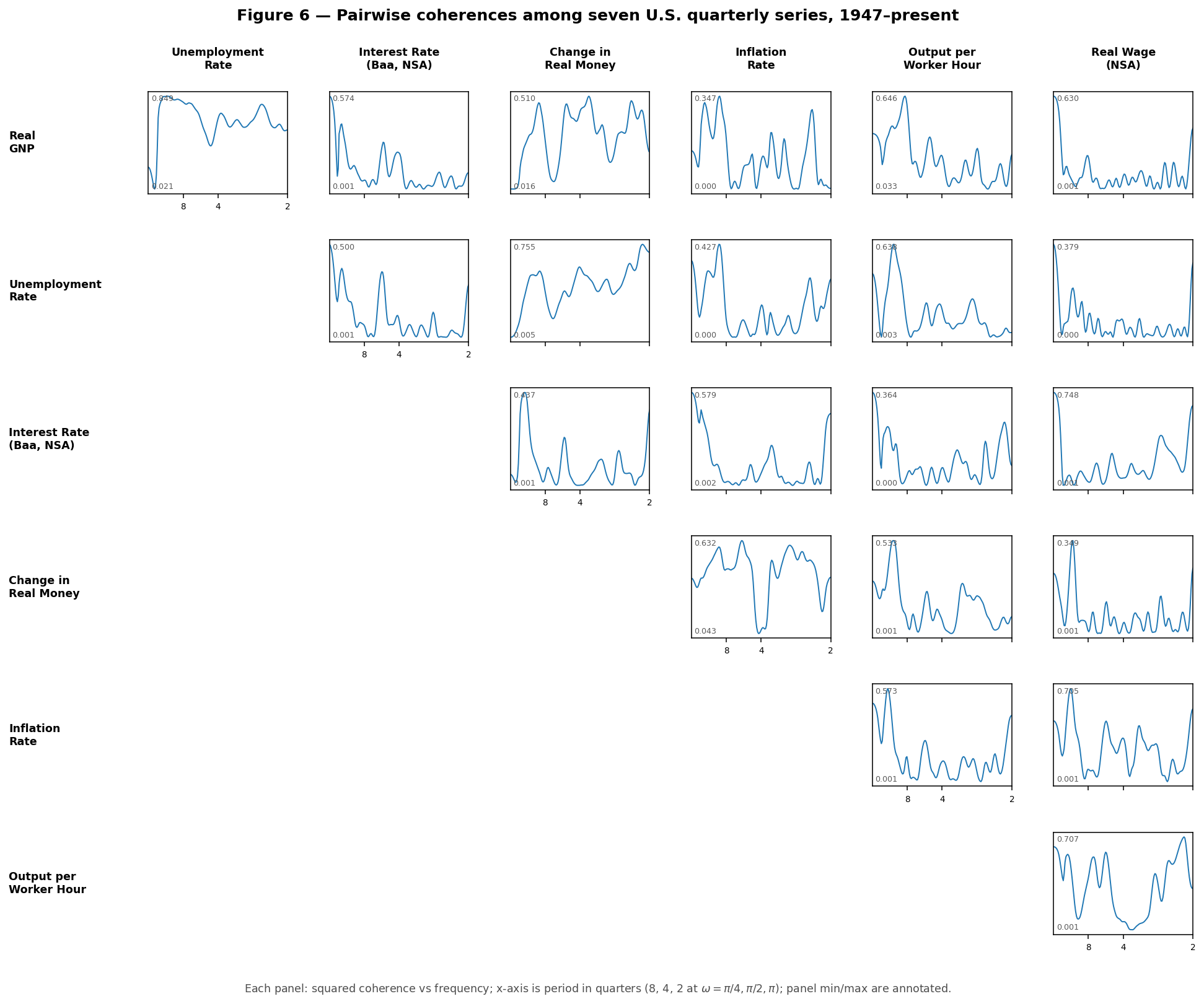
Fig. 14 Figure 6. Pairwise (magnitude-squared) coherences among the seven U.S. quarterly series, 1947–present (a modernized extension of Sargent’s original 1948:I–1976:IV figure). The panels form the upper triangle of the \(7\times 7\) coherence matrix; each is estimated from smoothed auto- and cross-periodograms of the linearly detrended series (smoothing is essential — the raw squared coherence of a single realization is identically one). The horizontal axis is the period \(2\pi/\omega\) in quarters (8, 4, 2 at \(\omega = \pi/4, \pi/2, \pi\)); each panel is auto-scaled to its own minimum and maximum, which are annotated. Real GNP, the unemployment rate, and output per worker hour show the highest coherences at the low (long-period) business-cycle frequencies — the empirical counterpart of the “business cycle as common movement” definition. Generated by code/fig6_coherences.py.

Note

Figures 5 and 6 here are modernized reproductions spanning 1947 to the present rather than Sargent’s original 1947–1975 / 1948–1976 windows. The qualitative lessons survive the longer sample: the “typical spectral shape” still dominates real GNP, unemployment, the Baa rate, output per hour, and the real wage, and the strongest low-frequency coherence remains that between real GNP and unemployment. Two caveats of the modernization: the series are quarterly averages, which mutes the seasonal peaks near four and two quarters that the text describes; and the 2020 COVID shock injects a large transient that is visible in several series and their spectra.