A Difficulty in Interpreting Vector Autoregressions#
Note
This section is based on Lars Peter Hansen and Thomas J. Sargent, “Two Difficulties in Interpreting Vector Autoregressions,” Chapter 4 of Rational Expectations Econometrics (Westview Press, 1991). That chapter describes two difficulties — one for discrete-time models and one arising from time aggregation of continuous-time models. We treat only the first, discrete-time difficulty (the paper’s Introduction and Section 1), and we set the sampling interval to \(\Delta = 1\) throughout, so that one period is one unit of time.
The equilibrium of a dynamic rational expectations model is a covariance stationary \((n\times 1)\) vector process \(z_t\). Surprises — random shocks to the agents’ information sets — prompt revisions in their plans and so move equilibrium prices and quantities. Since every covariance stationary process has a vector autoregression (Wold’s theorem of Representation Theory), it is tempting to summarize such an equilibrium by its vector autoregression and to read the innovation accounting of Sims (1980) — variance decompositions and impulse responses to the autoregression’s innovations — as though those innovations were the shocks hitting agents. This section describes a class of models in which that reading is wrong: the white noise a vector autoregression recovers is generally not the white noise that is fundamental for the agents, and innovation accounting, taken at face value, gives a distorted picture of how the economy responds to the agents’ surprises.
The vector autoregression and its innovations#
Let \(z_t\) be an \((n\times 1)\) covariance stationary process, observed at the integer dates \(t = 0, \pm 1, \pm 2, \dots\) (this is the paper’s setup with \(\Delta = 1\)). Its vector autoregression is the projection equation
where \(a_t\) is the \((n\times 1)\) vector of population regression residuals, with \(E a_t a_t^T = V\), determined by the orthogonality (normal-equation) conditions
and where the \(A_j\) are square summable, \(\sum_{j=1}^{\infty}\operatorname{tr}(A_j A_j^T) < \infty\). Conditions (436)–(437) make \(a_t\) a vector white noise, \(E a_t a_{t-j}^T = 0\) for \(j\neq 0\), that lies in the closed linear space spanned by \(\{z_t, z_{t-1}, \dots\}\). Eliminating the lagged \(z\)’s from (436) gives the vector moving-average (Wold) representation
whose coefficients satisfy \(A(L)\,C(L) = I\) with \(A(L) = I - \sum_{j\geq 1} A_j L^j\) and \(C(L) = \sum_{j\geq 0} C_j L^j\), and are square summable. Because \(a_t\) belongs to the space spanned by current and lagged \(z\)’s, it is a fundamental white noise for \(z_t\): current and lagged \(z\)’s reveal it. There are also non-fundamental representations \(z_t = \sum_j \tilde C_j\, \tilde a_{t-j}\) in which \(\{\tilde a_t, \tilde a_{t-1},\dots\}\) spans a strictly larger space than \(\{z_t, z_{t-1},\dots\}\); current and lagged \(z\)’s fail to be “fully revealing” about such an \(\tilde a_t\).
Representation (438) induces the decomposition of the \(j\)-step-ahead prediction-error covariance that underlies innovation accounting,
where \(\hat E\) is the linear least squares projection operator. Sims’s methods estimate the autoregression (436), form the moving average (438), and decompose (439) to attribute prediction-error variance to innovations in particular components of \(z_t\).
Now suppose the equilibrium of an economic model has its own moving-average representation in terms of the shocks to agents’ information sets,
where \(\epsilon_t\) is the white noise that is fundamental for the agents. The interpretive question is whether the vector-autoregression innovations \(a_t\) equal the agents’ shocks \(\epsilon_t\) — and whether the response coefficients \(C_j\) equal the economic responses \(D_j\). If they do, innovation accounting reads off the economics directly. The next subsection exhibits a class of models in which they do not.
Unrevealing models#
Consider models whose equilibrium solves the pair of stochastic difference equations
where \(y_t\) is \(n_1\times 1\), \(x_t\) is \(n_2\times 1\), \(H(L) = H_0 + \dots + H_{m_1}L^{m_1}\) and \(J(L) = J_0 + \dots + J_{m_2}L^{m_2}\) are matrix polynomials, \(K(L) = \sum_{j\geq 0} K_j L^j\) with \(K_0 = I\), and \(\epsilon_t = x_t - E(x_t\mid x_{t-1},x_{t-2},\dots)\) is the fundamental white noise of the forcing process \(x_t\). We assume the zeros of \(\det H(z)\) lie outside the unit circle, those of \(\det J(z)\) inside, and those of \(\det K(z)\) not outside. Interrelated factor-demand models of the Lucas–Prescott type are special cases with \(J(L^{-1}) = H(L^{-1})^T\); dominant-player and Kennan–Sargent market models give other cases.
Equation (441) is solved with the prediction technology of Linear Least Squares Prediction and the partial-fraction calculus of The Residue Theorem Behind Partial Fractions. Factor \(\det J(z^{-1}) = \lambda_0\prod_{j=1}^{k}(1-\lambda_j z^{-1})\), with \(k = m_2 n_1\) and the distinct \(\lambda_j\) inside the unit circle, and expand
Each term is a geometric sum of expected future \(x\)’s, evaluated with the Hansen–Sargent formula (the seasonal-lead calculation of Predicting Geometric Distributed Leads),
Summing over \(j\) and writing \(M(K(L)) = \sum_{j=1}^{k} M_j\, p\big(\frac{L K(L) - \lambda_j K(\lambda_j)}{L - \lambda_j}\big)\), the equilibrium becomes
The full vector \((y_t^T, x_t^T)^T\) — \(n_1 + n_2\) variables — is driven by only the \(n_2\) white noises \(\epsilon_t\), so it has a singular spectral density: the model fits an internal subset of equations with \(R^2 = 1\). To avoid this, suppose the econometrician observes only a subset \((y_t, x_{2t})\) of the variables, where \(x_t = (x_{1t}, x_{2t})\) and \(K(L) = \operatorname{diag}(K_1(L), K_2(L))\). Writing \(z_t = (y_t^T, x_{2t}^T)^T\) and \(\epsilon_t = (\epsilon_{1t}^T, \epsilon_{2t}^T)^T\), the observed system is
Equation (445) is a moving average expressing \(z_t\) in terms of the agents’ shocks \(\epsilon_t\). The shocks \(\epsilon_t\) are fundamental for the agents’ information set \((x_{1t}, x_{2t})\); the question is whether they are also fundamental for the econometrician’s data \(z_t = (y_t, x_{2t})\). By construction the econometrician’s space is contained in the agents’; the issue is whether it is as large. It is not, in general: \(\epsilon_t\) is fundamental for \(z_t\) if and only if the zeros of \(\det R(z)\) do not lie inside the unit circle, i.e.
and Hansen and Sargent (1980) exhibit a class of models — not thin in any natural sense — for which (446) fails.
When (446) fails, the Wold representation that a vector autoregression recovers is not (445). Instead there is a matrix polynomial \(G(L)^T = \sum_{j\geq 0} G_j^T L^j\), one-sided in nonnegative powers of \(L\), with \(G(L^{-1})G(L)^T = I\), that “flips” the inside-the-circle zeros of \(\det R(z)\) to the outside (a Blaschke factorization). Setting \(R^*(L) = R(L)\,G(L^{-1})\) and \(\epsilon_t^* = G(L)^T\epsilon_t\), the equilibrium can be re-expressed as
and now \(\epsilon_t^*\) is fundamental for \(z_t\): (447) is the Wold representation, and \(\epsilon_t^* = R^*(L)^{-1} S(L) z_t\) is recovered by the vector autoregression. The Wold innovation \(\epsilon_t^*\) is a one-sided distributed lag of current and past \(\epsilon_t\)’s, \(\epsilon_t^* = G(L)^T\epsilon_t\) — it mixes the agents’ current surprise with old news. Only when no zeros of \(\det R(z)\) lie inside the unit circle can \(G(L)^T\) be taken to be the identity and \(\epsilon_t^* = \epsilon_t\). Otherwise the two white noises differ, and their contemporaneous covariances obey the strict inequality
the contemporaneous innovation the econometrician sees carries more variance than the agents’ contemporaneous surprise, because the econometrician’s innovation has folded in past shocks that the agents already knew.
A numerical example: price and quantity in a single market#
A useful illustration is a single market in which the econometrician observes only the \(2\times 1\) vector \(y_t = (q_t, p_t)\) of quantity and price — there are no separately observed forcing variables \(x_t\), so (445) specializes to \(H(L)y_t = M(C_1(L))\epsilon_{1t}\).
A representative supplier and a representative demander each solve a linear-quadratic dynamic problem, and their first-order (Euler) conditions are
where (449) is the supply Euler equation of a competitive firm with quadratic costs of adjusting output (in \((1-L)q_t\)), (450) is the demand Euler equation with \(a(L) = a_0 + a_1 L + a_2 L^2 + a_3 L^3 + a_4 L^4\) describing a durable-services technology, \(\beta\) is the discount factor, and \(s_t, d_t\) are serially correlated supply and demand shocks,
with \(B_s(z), B_d(z)\) having zeros outside the unit circle and \(w_{st}, w_{dt}\) mutually uncorrelated white noises that agents observe. Setting \(y_t = (q_t, p_t)\), \(\epsilon_t = (w_{st}, w_{dt})\), \(K_2(L) = 0\), and \(K_1(L) = \operatorname{diag}(B_s(L), B_d(L))\), the model is a member of the class (441). Eliminating \(p_t\) between (449) and (450) gives a single Euler equation in \(q_t\) whose two-sided characteristic operator factors as \(J(L^{-1})H(L) = E(L)\), where
with the zeros of \(\det J(z)\) inside and those of \(\det H(z)\) outside the unit circle. The equilibrium then has the two representations
with \(S(L) = H(L)\) and \(R(L) = M(C_1(L))\). For this market the zeros of \(\det R(z)\) lie inside the unit circle, so (446) fails and the two white noises differ.
We compute the example with the parameters
To solve the model we map it into the class of linear-quadratic economies of Hansen and
Sargent (2013) — the construction in the paper’s appendix — and use QuantEcon’s DLE
(dynamic linear economy) class, which solves the optimal resource-allocation problem by
dynamic programming and returns the state-space equilibrium \(x_{t+1} = A^o x_t + C w_{t+1}\),
\(z_t = G x_t\). Impulse responses to the agents’ structural shocks are read directly off this
system; the Wold representation (447) and its innovations \(\epsilon_t^*\) are obtained
by passing the equilibrium through the Kalman filter (the innovations representation), and the
filter that maps \(\epsilon_t \mapsto \epsilon_t^*\) is the whitener. The figure below
collects the results.
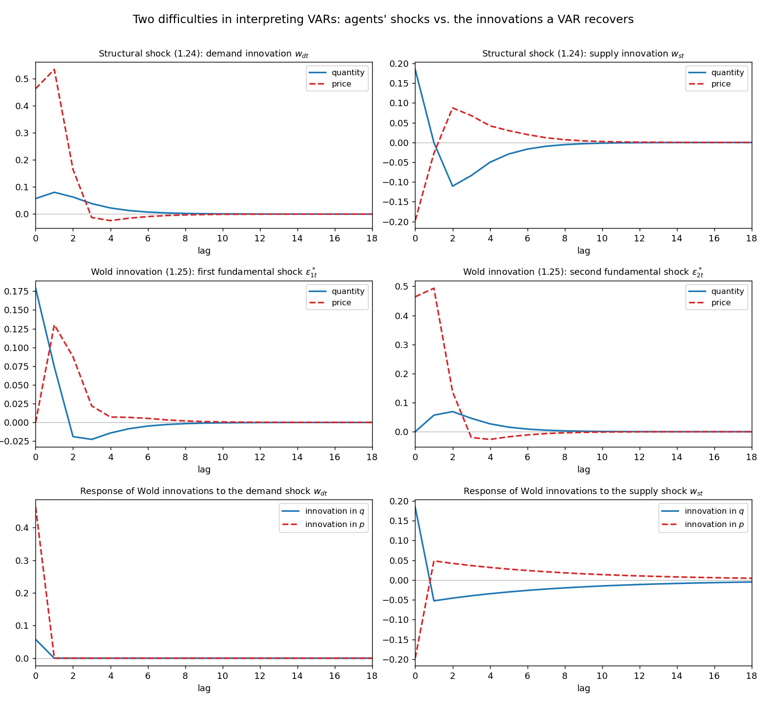
Fig. 24 Figure. The single-market example of Hansen and Sargent (1991). Row 1 — the response
of quantity and price to the agents’ structural shocks (representation (452),
left): a demand surprise sends price up sharply on impact with little quantity response, while
a supply surprise sends quantity and price off in opposite directions. Row 2 — the response
to the Wold innovations a vector autoregression recovers (representation (452),
right, with \(q\) ordered first in the Gram–Schmidt orthogonalization). Row 3 — the response
of the Wold innovations \(\epsilon_t^*\) to the structural shocks (\(\epsilon_t^* =
G(L)^T\epsilon_t\)): the demand surprise is impounded almost contemporaneously (mostly in the
price innovation), but the supply surprise enters the recovered innovations as a distributed
lag. The recovered innovations are therefore mixtures of current and past structural shocks,
not the structural shocks themselves. Computed with QuantEcon’s DLE class (a port of the
authors’ MATLAB twodiff1.m); see
code/ch36a_two_difficulties.py.#
The economic reading of the rows is the substance of the example. The supply innovation \(w_{st}\) shows up in the recovered innovations only as a distributed lag (Row 3, right), because the slow adjustment of quantity means that a supply surprise is revealed to the econometrician gradually, through the path of \((q_t, p_t)\), rather than all at once. The demand innovation \(w_{dt}\), by contrast, hits price almost contemporaneously (Row 3, left), so the price innovation in the autoregression is a fairly timely indicator of the demand surprise — but the quantity innovation is a long distributed lag, mainly of the supply surprise. An econometrician who interpreted the autoregression’s innovations as the agents’ shocks would therefore misattribute the timing and the sources of the market’s response.
The covariance inequality (448) is the quantitative signature of the discrepancy. For this parameterization the contemporaneous covariance of the recovered (Wold) innovations exceeds that of the agents’ structural innovations,
confirming that the innovation the econometrician sees carries more contemporaneous variance than the agents’ surprise — it has folded in shocks that the agents already knew. None of this can be detected from the autoregression alone; it takes the cross-equation restrictions of the economic theory, estimated as in Hansen and Sargent (1980), to recover \(R(L)\) — and hence the agents’ shocks \(\epsilon_t\) — from a record on \((q_t, p_t)\), even when some zeros of \(\det R(z)\) lie inside the unit circle.
The moral for innovation accounting
A vector autoregression always recovers some fundamental white noise \(a_t\) for the observed \(z_t\), and Sims’s innovation accounting always produces a tidy variance decomposition. But the fundamental noise for the data need not be the fundamental noise for the agents. When it is not — as in this market, where quantity adjusts sluggishly and so reveals supply surprises only with a lag — the impulse responses and variance decompositions describe the data’s own internal forecasting structure, not the economy’s response to the surprises that actually move agents. Reading economic meaning into them requires the restrictions of a model, not just the autoregression.
Dynamic supply and demand curves#
It is illuminating to solve the supplier’s and the demander’s Euler equations (449)–(450) separately, before imposing market clearing. Each is an expectational difference equation in \(q_t\), and each is solved by the now-standard device of Chapter IX — Difference Equations and Lag Operators and Predicting Geometric Distributed Leads: factor the characteristic operator into a stable root and an unstable root, solve the stable root backwards into a feedback on lagged quantities, and solve the unstable root forwards into a geometric sum of expected future variables. The two solutions are dynamic supply and demand curves.
The dynamic supply curve. Write the supplier’s Euler equation (449) as \(E_t\,\phi_s(L)\,q_t = p_t - s_t\), with characteristic operator \(\phi_s(L) = h_s + g_s(1-\beta L^{-1})(1-L)\). Because \(\phi_s\) is symmetric under \(L \mapsto \beta L^{-1}\), the roots of its symbol come in a reciprocal pair \((\delta_s,\ \beta/\delta_s)\), the two solutions of the supplier’s characteristic equation
Let \(\delta_s\) be the smaller root, \(|\delta_s| < \sqrt{\beta} < 1\) (for the chapter’s parameters \(\delta_s \approx 0.709\)). Then \(\phi_s\) factors as
an unstable forward factor \((1-\delta_s L^{-1})\), with \(|\delta_s| < 1\), and a stable backward factor \((1-\tfrac{\delta_s}{\beta}L)\), with \(|\delta_s/\beta| < 1\). Solving the forward root forward — a geometric sum of expected future variables, exactly as in Predicting Geometric Distributed Leads — and reading the backward root as a feedback on the lag of \(q\), the supplier’s Euler equation becomes the dynamic supply curve
Current quantity supplied is a geometrically declining feedback on its own lag \(q_{t-1}\) plus the conditional expectation of a discounted geometric sum of future prices \(p_{t+j}\) and future supply shocks \(s_{t+j}\), discounted at the rate \(\delta_s\). Higher expected future prices raise current supply (the curve slopes up in the price path); a higher expected cost shock \(s_{t+j}\) lowers it. Only the single lag \(q_{t-1}\) appears, because the supplier’s adjustment cost penalizes \((1-L)q_t\) one period at a time.
The dynamic demand curve. The demander’s Euler equation (450) is \(E_t\,\phi_d(L)\,q_t = -(p_t + d_t)\), with characteristic operator \(\phi_d(L) = h_d + g_d\,a(\beta L^{-1})\,a(L)\). Since \(a(L)\) has degree four, \(\phi_d\) is again symmetric under \(L \mapsto \beta L^{-1}\), but now its symbol has eight roots in four reciprocal pairs \((\delta_{d,i},\ \beta/\delta_{d,i})\), \(i = 1,\dots,4\) (for the chapter’s parameters the four stable \(\delta_{d,i}\) are two complex-conjugate pairs of modulus \(\approx 0.30\) and \(\approx 0.39\)). Collecting the four stable roots \(|\delta_{d,i}| < \sqrt{\beta}\), the factorization is
with \(\nu_d > 0\) a normalizing constant and \(c_d(\beta L^{-1}) = \prod_i(1 - \delta_{d,i}L^{-1})\) the forward factor. Inverting the forward factor with a partial-fraction expansion (The Residue Theorem Behind Partial Fractions),
and reading the backward factor \(c_d(L)\) as a feedback on lags, the demander’s Euler equation becomes the dynamic demand curve
Now current quantity demanded depends on four lags \(q_{t-1},\dots,q_{t-4}\) — the demander’s durable-services technology \(a(L)\) spreads adjustment over four periods — and on a sum of geometric feedforward terms, one per stable root \(\delta_{d,i}\), each a discounted sum of future prices and future demand shocks. (The \(\delta_{d,i}\) come in conjugate pairs, so the weights combine into real, damped-oscillatory coefficients.) The price terms enter with a negative sign: higher expected future prices lower current demand, so the demand curve slopes down in the price path.
Both shocks shift both curves. Taken at face value, the dynamic supply curve (455) seems to involve only supply shocks \(s_{t+j}\), and the dynamic demand curve (457) only demand shocks \(d_{t+j}\). But each curve also contains the conditional expectations \(E_t\,p_{t+j}\) of future prices, and in equilibrium the price process is driven by both shocks. A demand surprise that moves expected future prices therefore shifts the dynamic supply curve through its term \(E_t\sum_j \delta_s^{\,j} p_{t+j}\), and a supply surprise that moves expected future prices shifts the dynamic demand curve through its terms \(E_t\sum_j \delta_{d,i}^{\,j} p_{t+j}\). It is exactly this dependence on forecasts of future prices — absent from static supply and demand curves — that couples the two sides of the market and makes the equilibrium dynamics richer than a sequence of momentary intersections.
Equilibrium. The rational expectations equilibrium equates quantity demanded to quantity supplied period by period. Imposing \(q_t^{\text{supply}} = q_t^{\text{demand}} = q_t\) in (455) and (457), and requiring that the price forecasts \(E_t\,p_{t+j}\) that appear in both curves be the ones generated by the equilibrium price process itself, pins down the joint \((q_t, p_t)\) process. That equilibrium is precisely the structural representation \(S(L)\,(q_t, p_t)^T = R(L)\,(w_{dt}, w_{st})^T\) of (452) — the one whose innovations a vector autoregression generally fails to recover.
Each side of the market as a price-taking linear regulator#
The dynamic supply and demand curves are the first-order conditions of two distinct optimization problems — one solved by the representative supplier, one by the representative demander — and in the rational expectations equilibrium both agents are price takers. We now make those problems explicit and cast each as a discounted optimal linear regulator in which the agent faces the equilibrium price as an exogenous stochastic process. This is an instance of the “Big \(X\), little \(x\)” (or “Big \(K\), little \(k\)”) device used throughout modern macroeconomics, and the recursive set-up is the one followed in Section 50.7.1, “Recursive formulation of a follower’s problem,” of the QuantEcon dynamic Stackelberg lecture: append the exogenous aggregate law of motion to the agent’s own state, and solve an ordinary linear regulator.
The two optimization problems. The representative supplier chooses \(\{q_t\}\) to maximize
taking the market price \(\{p_t\}\) as given (and observing its cost shock \(s_t\)): it earns revenue \(p_t q_t\), pays a quadratic cost of adjusting output, and is buffeted by \(s_t\). The representative demander chooses \(\{q_t\}\) to maximize
again taking \(\{p_t\}\) as given: it pays \(p_t q_t\) for the good, values the service flow \(a(L)q_t\) generated by current and past purchases, and is shifted by \(d_t\). Differentiating (458) and (459) with respect to \(q_t\) returns exactly the supplier’s and demander’s Euler equations (449) and (450).
The exogenous price process (Big \(X\)). In a rational expectations equilibrium each agent’s
forecasts of future prices must be model-consistent — they must be the forecasts implied by the
equilibrium price process, which is the one the Hansen–Sargent DLE computed above. Write
that equilibrium in state-space form,
with \(A = A^o\), \(C\), and the price selector \(G_p = M_c\) taken directly from the DLE solution
(the supply and demand shocks are linear in the same state, \(s_t = G_s X_t\) and \(d_t = G_d
X_t\)). A price-taking agent treats \(X_t\) as an exogenous Markov state it cannot influence. The
key consequence is that, because \(X_t\) is Markov, every conditional expectation of a future
price is a linear function of the current state,
so the geometric feed-forward sums \(E_t\sum_j \delta^{\,j} p_{t+j}\) in the dynamic supply and demand curves collapse into linear functions of \(X_t\).
The recursive formulation. Following Section 50.7.1 of the dynamic Stackelberg lecture, we append the exogenous law of motion (460) to the agent’s own state and solve an optimal linear regulator. For the supplier, the composite state stacks the aggregate price-process state \(X_t\) (“Big \(X\)”) on top of the supplier’s own lagged quantity \(q_{t-1}\) (“little \(x\)”), \(\widehat X_t = (X_t^{\,\prime}, q_{t-1})'\), and evolves as
The block-triangular transition makes \(X_t\) exogenous — the supplier’s choice \(q_t\) cannot move it — while \(q_t\) becomes next period’s lag. Writing the one-period return (458) as a quadratic form in \((\widehat X_t, q_t)\) (using \(p_t = G_p X_t\), \(s_t = G_s X_t\)), the supplier solves a standard discounted linear regulator, and its optimal policy is the feedback rule
The coefficient on the supplier’s own lag is the stable root \(\delta_s/\beta\) of the supply curve (455), and — by (461) — the feed-forward \(-F_X X_t\) is exactly the geometric sum \(\frac{\delta_s}{g_s\beta}E_t\sum_j \delta_s^{\,j}(p_{t+j}-s_{t+j})\) written as a linear function of the state. The demander’s regulator has the same shape with a richer own state \((q_{t-1},\dots,q_{t-4})\) — four lags, because the services technology \(a(L)\) spreads adjustment over four periods — and its feedback on those four lags reproduces the coefficients \(\gamma_{d,k}\) of the demand curve (457).
Solving the two regulators with QuantEcon’s LQ routine, facing the DLE equilibrium price
process \((A, C, G_p)\), returns precisely the dynamic-curve coefficients: the supplier’s feedback
on \(q_{t-1}\) is \(\delta_s/\beta = 0.744\), and the demander’s feedback on \((q_{t-1},\dots,q_{t-4})\)
is \((\gamma_{d,1},\dots,\gamma_{d,4}) = (-0.117,\,-0.079,\,-0.045,\,-0.017)\) — exactly the
coefficients read off the factored Euler equations. See
code/ch36a_price_taker_lq.py.
Big \(X\) equals little \(x\): the equilibrium fixed point. Each agent’s rule is a best response
to the price process \(X_t\), and only a best response: the agent takes \(X_t\) as given, and its
own little-\(x\) choice does not move Big \(X\). What closes the model is the requirement — the heart
of the “Big \(X\), little \(x\)” trick — that the aggregate the agents respond to be consistent with
the aggregate their choices produce. Here that means the market clears, \(q_t^{\text{supply}} =
q_t^{\text{demand}}\), at the common price, and the price process \(X_t\) that both agents forecast
is the very process those market-clearing quantities generate. The Hansen–Sargent DLE computes
exactly this fixed point: its equilibrium price process is the one for which the suppliers’ and
demanders’ price-taking best responses clear the market period by period. Feeding that process
back into either agent’s regulator — as the verification does — returns a quantity rule
consistent with it.
Open-loop versus closed-loop decision rules. The construction has produced two distinct pairs of decision rules. We keep them apart. The dynamic supply curve (455) and the dynamic demand curve (457) give each agent’s optimal quantity as a function of its own past quantities and of its forecasts \(E_t\,p_{t+j}\) of an arbitrary price process \(\{p_t\}_t\) that it takes as exogenously given. They are best responses to whatever price process the agent happens to face, and they assume nothing about how that price is generated — in particular, they do not assume it is produced by the market the agent trades in. In this sense (455) and (457) are an open-loop pair: the loop between the market’s quantity and its price is left open, and the rules are valid outside any particular rational expectations equilibrium. The regulator feedback rules \(q_t = -F\,\widehat X_t\) are a different pair. They are the same optimizing behavior with the equilibrium price process (460) substituted in: evaluating the feed-forward sums with \(E_t\,p_{t+j} = G_p A^{\,j} X_t\) collapses each open-loop curve into a feedback on the equilibrium state \(X_t\) (together with the agent’s own lags). These are a closed-loop pair — the price each agent responds to is now the very one the equilibrium system produces, so the market-clearing loop is closed — and they are the supply and demand decision rules that obtain inside the rational expectations equilibrium. Equivalently, (455)–(457) are the outside-an-REE pair of rules and \(q_t=-F\widehat X_t\) the inside-an-REE pair. The two coincide only after one fixes the price process to be the equilibrium one; passing from the open-loop curve to the closed-loop rule — from outside the REE to inside it — is exactly the act of imposing rational expectations on the agents’ price forecasts.
The key lesson. Whichever representation one adopts — the open-loop supply and demand curves (455)–(457) or their closed-loop counterparts \(q_t = -F\,\widehat X_t\) — both deliver the same message: each decision maker’s quantity today depends not on today’s price alone but on the entire prospective continuation path of the product price, \(\{p_{t+j}\}_{j\ge 0}\), forecast from today out into the indefinite future. In the open-loop curves the dependence is explicit, through the discounted geometric sums \(E_t\sum_{j\ge 0}\delta^{\,j}\,p_{t+j}\) of expected future prices; in the closed-loop rules it is encoded in the feedback on the equilibrium state \(X_t\), which carries exactly those forecasts via \(E_t\,p_{t+j} = G_p A^{\,j} X_t\). Either way, supply and demand are inescapably forward-looking: current decisions are governed by the whole expected future path of prices, not by the current price in isolation. And because that equilibrium price path is itself driven by both disturbances, both pairs of rules make each side’s quantity depend on both shock processes: the supply shock \(s_t\) and the demand shock \(d_t\) each appear in the dynamic supply curve and in the dynamic demand curve alike. Today’s suppliers and today’s demanders both react to supply and demand shocks — through their common effect on the prospective path of prices.
References#
Lars Peter Hansen and Thomas J. Sargent. Formulating and estimating dynamic linear rational expectations models. Journal of Economic Dynamics and Control, 2(1):7–46, 1980.
Lars Peter Hansen and Thomas J. Sargent. Two difficulties in interpreting vector autoregressions. In Rational Expectations Econometrics, chapter 4. Westview Press, Boulder, CO, 1991.
Lars Peter Hansen and Thomas J. Sargent. Recursive Models of Dynamic Linear Economies. Princeton University Press, Princeton, NJ, 2013.
Thomas J. Sargent and John Stachurski. Dynamic stackelberg problems. QuantEcon lecture. https://python-advanced.quantecon.org/dyn_stack.html.
Christopher A. Sims. Macroeconomics and reality. Econometrica, 48(1):1–48, 1980.